Plotting (Good) Exercises
Exercise 1
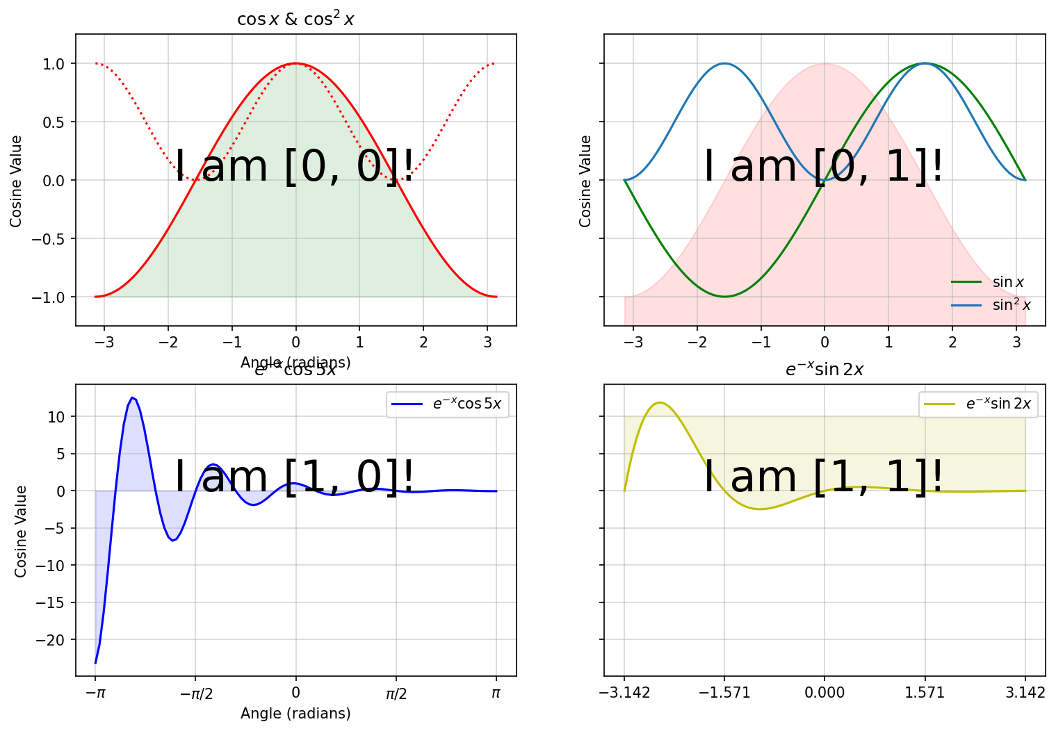
Before
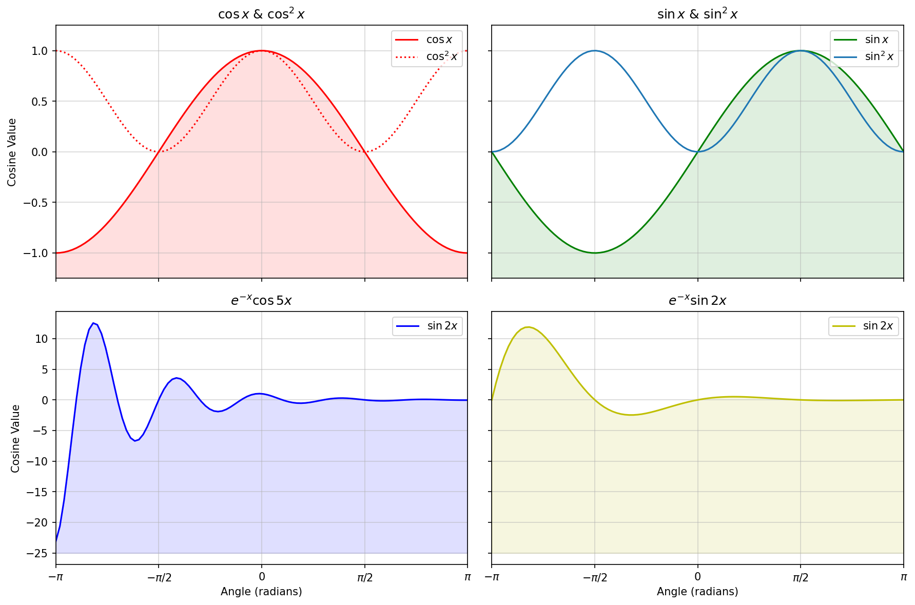
After
The code shown in the Code tab generates the ‘Before’ figure shown in the Plots tab.
Your task is to modify this code to end with the ‘After’ figure in jpg format.
Here are some things to get you started:
- Remove the text ‘I am..’
- Change the colours used for filling.
- Change the limits of the filled areas.
- Add titles to each subplot.
- Share the x axis across columns.
- Add/Remove labels to the x-axis.
- Make the tick labels of the two bottom plots the same.
- Add grids to all subplots.
- Add a legend to all subplots in the upper right position.
- Use
tight_layout()to improve the figure. - Save the figure as a
jpgfile.
You might want to view the images in their full resolution by opening them in another tab.
#--------- Generate cosine and sine values --------#
x = np.linspace(-np.pi, np.pi, num=100, endpoint=True)
cos_x = np.cos(x)
sin_x = np.sin(x)
fun1_x = np.exp(-x) * np.cos(5 * x)
fun2_x = np.exp(-x) * np.sin(2 * x)

#------- Plot the data -------#
fig, axes = plt.subplots(nrows=2, ncols=2,
                         figsize=(12, 8),  sharey='row')

#------- Subplot 1 -------#
axes[0, 0].plot(x, cos_x, color='r', label='$\cos x$')
axes[0, 0].plot(x, cos_x**2, color='r',
                linestyle=':', label='$\cos^2 x$')
axes[0, 0].set_title('$\cos x$ & $\cos^2x$')
axes[0, 0].set_ylabel('Cosine Value')
axes[0, 0].fill_between(x, cos_x, -1, color='g', alpha=.125)
axes[0, 0].set_xlabel('Angle (radians)')
axes[0, 0].text(0, 0, 'I am [0, 0]!', fontsize=30,
                horizontalalignment='center')

#------- Subplot 2 -------#
axes[0, 1].plot(x, sin_x, color='g', label='$\sin x$')
axes[0, 1].fill_between(x, cos_x, -2, color='r', alpha=.125)
axes[0, 1].plot(x, sin_x**2, label='$\sin^2 x$')
axes[0, 1].set_ylabel('Cosine Value')
axes[0, 1].set_ylim(-1.25, 1.25)
axes[0, 1].legend(loc='lower right', frameon=False)
axes[0, 1].text(0, 0, 'I am [0, 1]!', fontsize=30,
                horizontalalignment='center')

#------- Subplot 3 -------#
axes[1, 0].plot(x, fun1_x, color='b', label='$e^{-x}\cos 5x$')
axes[1, 0].fill_between(x, fun1_x, 0, color='b', alpha=.125)
axes[1, 0].set_title('$e^{-x}\cos 5x$')
axes[1, 0].set_xlabel('Angle (radians)')
axes[1, 0].set_ylabel('Cosine Value')
axes[1, 0].set_xticks([-np.pi, -np.pi / 2, 0, np.pi / 2, np.pi])
axes[1, 0].set_xticklabels(['$-\pi$', '$-\pi/2$', '0', '$\pi/2$', '$\pi$'])
axes[1, 0].legend()
axes[1, 0].text(0, 0, 'I am [1, 0]!', fontsize=30,
                horizontalalignment='center')

#------- Subplot 4 -------#
axes[1, 1].plot(x, fun2_x, color='y', label='$e^{-x}\sin 2x$')
axes[1, 1].set_title('$e^{-x}\sin 2x$')
axes[1, 1].fill_between(x, fun2_x, 10, color='y', alpha=.125)
axes[1, 1].set_xticks([-np.pi, -np.pi / 2, 0, np.pi / 2, np.pi])
axes[1, 1].legend()
axes[1, 1].text(0, 0, 'I am [1, 1]!', fontsize=30,
                horizontalalignment='center')

# 'flatten', 'opens' the 2D array into a simple 1D array
for a in axes.flatten():
    a.grid(alpha=.5)

# plt.tight_layout()
plt.show(block=False)