08| All about plotting

Introduction

This challenge is about visualizing mathematical functions and vectors.

A quick primer in vectors

What are vectors?

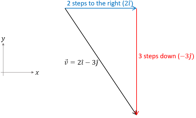
In case you need a reminder, we begin this problem with a recap on vectors. To put it simply, a vector is a physical quantity which consists of both magnitude and direction. Pictorially, vectors are represented by arrows, where the length of the arrow represents the magnitude and the arrowhead represents the direction. Mathematically, a vector can be represented through a combination of numbers and unit vectors (mathematical objects used to represent directions). For example, a vector \(\vec{v}\) can be written as: \[ \vec{v} = 2\hat{i} - 3\hat{j} \] where \(\hat{i}\) and \(\hat{j}\) are unit vectors in the \(x\)- and \(y\)-axes, respectively. Physically, we can interpret \(\vec{v}\) as an arrow which is equivalent to 2 steps in the direction of the positive x-axis, 3 steps in the direction of the negative y-axis. We say that 2 is the \(x\)-component of \(\vec{v}\) while -3 is the \(y\)-component of \(\vec{v}\). The figure below illustrates this physical picture.

Visualising vectors

One way to visualise vectors using Python is streamplot(). streamplot() is a function in matplotlib that draws the streamlines of a vector field. In simple terms, streamplot gives us the directions of vectors at different coordinates. It allows us to visualise many real-life phenomena including river flow, neural network, molecular velocity, and many others. This problem serves as an introduction to streamplot.

Familiarise yourself with streamplot(). You may read the write-up on streamplot on the matplotlib website as a start. Note that the write-up assumes that the vectors to be plotted are velocities, but all other vectors can be plotted the same way.

Tasks

1. Using streamplot(), produce a figure where all the vectors are pointing towards the origin.

2. Use streamplot(), to visualise the vector field \[ \vec{v}(x,y) = y\hat{i}-x\hat{j} \] Please adjust the relevant Matplotlib parameters for clear visualization.

3. The following equation describes the velocity of a fluid flowing around a cylinder of radius \(R\). \(U\) is the fluid’s initial speed, which is considered constant.

   \[ \begin{matrix} v_x = U\left(1-\dfrac{R^2}{x^2+y^2}\right) & \text{and} & v_y = -U\left(\dfrac{2R^2 y}{x^2+y^2}\right) \end{matrix} \]

   Visualise this flow pattern.
   Remember to adjust the relevant Matplotlib parameters for a clear visualisation.