from skimage import io
from skimage.color import rgb2grey
img_original = io.imread('three-circles.png')
img_grey = rgb2grey(img_original)
fig, ax = plt.subplots(nrows=1, ncols=2, figsize=(8, 4))
ax_original, ax_grey = ax
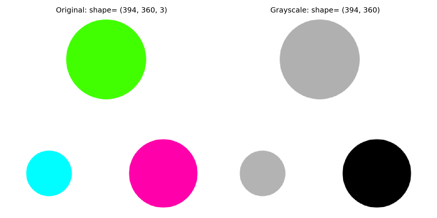
ax_original.imshow(img_original)
ax_original.set_title(f'Original: shape={img_original.shape}')
ax_grey.imshow(img_grey, cmap='gray')
ax_grey.set_title(f'Grayscale: shape={img_grey.shape}')
for a in ax.flat:
a.axis('off')Image Analysis (Good)

What to expect in this chapter
In this chapter, I will show you how to perform segmentation analysis, where you try to identify features of an image. It is one of the most important sub-fields under image analysis. It is the starting point of most detection algorithms, be it an image of a cell, an MRI scan of a brain, or an aerial photograph from a military drone. In this chapter, I will use the tools from scikit-image to discuss the basics of segmentation analysis.
1 scikit-image
scikit-image is a powerful image analysis package. You can install it by:
conda install anaconda::scikit-image2 Segmentation Analysis
Some typical steps go into extracting information from an image. These are:
- Convert the image to grayscale.
- Find and apply a threshold to binarise
- Identify and label objects
- Apply measurement tools to extract information about the objects
I will use the image three-circles.png and the tools from scikit-image to demonstrate these.
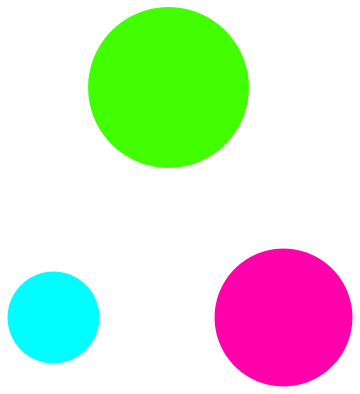
2.1 Convert the image to grayscale
Grayscale images (with just one layer) are more straightforward to analyze than RGB ones (with three layers). This is because a grayscale image has the same RGB values for each pixel. So, the first step is to convert the image into grayscale.
2.2 Binarise
Thresholding, or binarising, converts an image into black and white depending on what features you want to analyse. For example, to separate the foreground (our subject, such as a cell) from the background.
The threshold(\(t\)) separates the image into background and foreground. I.e., everything below (\(<t\)) will be black, and those values equal or above (\(\geq t\)) will be white.
Finding a threshold
scikit-image offers some functions to help us find a threshold. You can pick one (I will try Otsu and Yen) or try all. Here is how it works.
from skimage.filters import threshold_otsu, threshold_yen

img_original = io.imread('three-circles.png')
img_grey = rgb2grey(img_original)

print('{threshold_otsu(img_grey)=}')
print('{threshold_yen(img_grey)=}')
We can also try all the available methods using try_all_threshold()!
from skimage.filters import try_all_threshold

fig, ax = try_all_threshold(img_grey, figsize=(10, 8), verbose=False)
plt.show()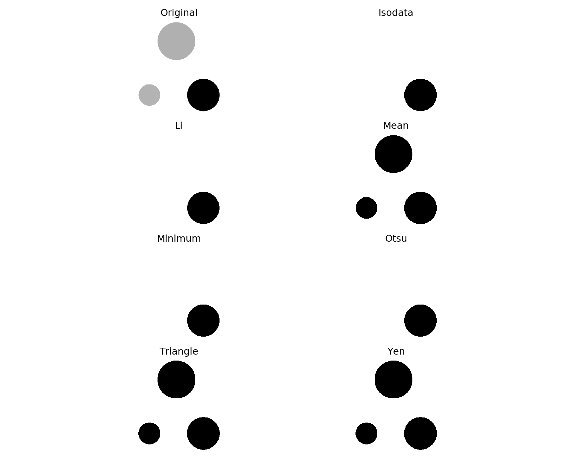
Yen seems to be the best.
Applying a threshold
Once we have a threshold, we can apply it to binarise the image.
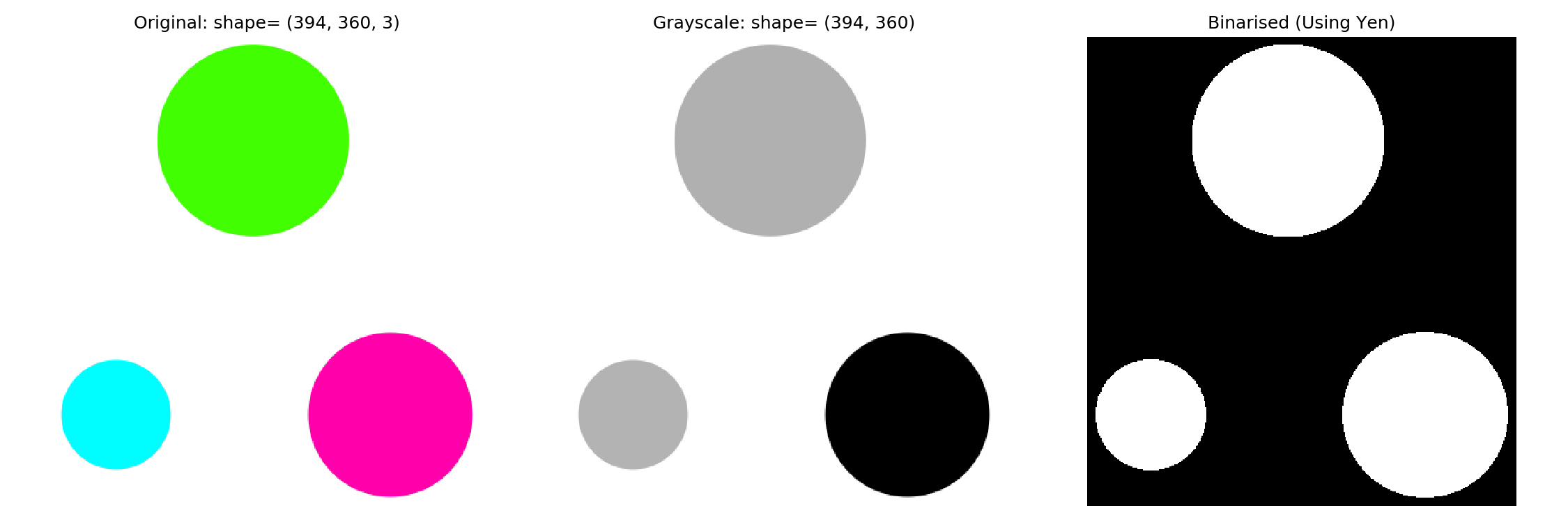
threshold = threshold_yen(img_grey)
img_binarised = img_grey < threshold

fig, ax = plt.subplots(nrows=1, ncols=3, figsize=(9, 3))
ax_original, ax_grey, ax_binarised = ax

ax_original.imshow(img_original)
ax_original.set_title(f'Original: shape= {img_original.shape}')

ax_grey.imshow(img_grey, cmap='gray')
ax_grey.set_title(f'Grayscale: shape= {img_grey.shape}')

ax_binarised.imshow(img_binarised, cmap='gray')
ax_binarised.set_title(f'Binarised (Using Otsu)')
2.3 Labelling
Note that skimage function measure.label() requires an image of type int
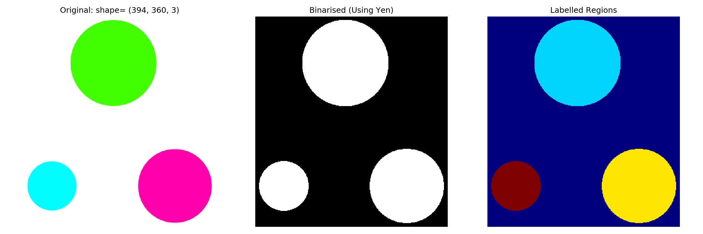
Once you have a binarised image, we can label features. More specifically, labeling ‘fills’ connected areas with an integer. For example, if you have three distinct regions, one will be filled with 1s, the next with 2s, and the third with 3s. This enables us to visualize the segments by a simple heat map.
Let me first show you what happens. I will then explain a bit more.
# measure.label() requires an image of type int
img_labelled = measure.label(img_binarised.astype('uint8'))

fig, ax = plt.subplots(nrows=1, ncols=3, figsize=(9, 3))
ax_original, ax_binarised, ax_labelled = ax

ax_original.imshow(img_original)
ax_original.set_title(f'Original: shape= {img_original.shape}')

ax_binarised.imshow(img_binarised, cmap='gray')
ax_binarised.set_title(f'Binarised (Using Yen)')

# Using jet to colour the different regions
ax_labelled.imshow(img_labelled, cmap='jet')
ax_labelled.set_title(f'Labelled Objects')
Making sense of labelling
I mentioned that labeling simply ‘fills’ distinct regions with integer numbers. This means we should be able to use masking to isolate these regions.
1st region
img_masked = img_labelled == 1
plt.imshow(img_masked)
2nd region
img_masked = img_labelled == 2
plt.imshow(img_masked)
3rd region
img_masked = img_labelled == 3
plt.imshow(img_masked)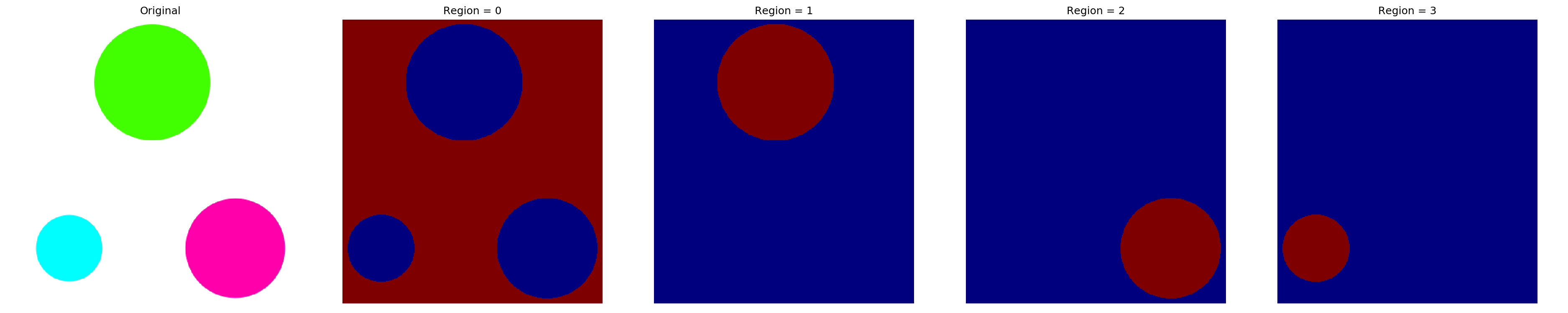
2.4 Measuring
Now that we have separated and labelled the regions, we can measure important characteristics (e.g. area, centroid) of these regions. Let me show you how.
---------- Region 0 ----------
Centre  : (87.0, 168.0)
Area    : 20565


---------- Region 1 ----------
Centre  : (317.0, 283.0)
Area    : 15193


---------- Region 2 ----------
Centre  : (317.0, 53.0)
Area    : 6793
# measure.label() requires an image of type int
img_labelled = measure.label(img_binarised.astype('uint8'))
region_info = measure.regionprops(img_labelled)
no_of_regions = len(region_info)
for count, region in enumerate(region_info):
print('-'*10, f'Region {count}', '-'*10)
print(f'Centre\t: {region.centroid}')
print(f'Area\t: {region.area}') # What is the area
print('\n')There are many more properties you can measure. Please see here for more information.