12| Monte Carlo Integration
Introduction
Evaluating integrals is necessary for most scientific modelling. So, many different integration methods have been developed. The Monte Carlo(MC) integration method is one of the most versatile. One of its charms is its ability to be scaled up to higher dimensions without much fuss. In this question, you will develop code to realise Monte Carlo integration.
Tasks
Area first
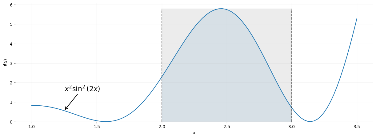
The image shows a plot of the function \(f(x)=x^2\sin^2(2x)\). Let’s try to estimate the area of the region shaded in blue.
Here is what you should do:
- Generate \((x,y)\) coordinates for a large number (\(n_\text{all}\)) of random points to evenly cover the area shaded in grey.
- As you can see, this region is defined by \(2 \le x \le 3\) and \(0 \le y\le 6\).
- Consider using
uniform()for this.
- Ask how many points you generated are below the curve (and therefore in the blue region). Let’s call this number \(n_\text{below}\).
- Notice that all random points in the blue region satisfy \(y_i \leq f(x_i)\)
- Now we can calculate the area of the blue region because: \[ \dfrac{\text{Blue Area}}{\text{Grey Area}} \approx \dfrac{n_\text{below}}{n_\text{all}}\Rightarrow \text{Blue Area}=\dfrac{n_\text{below}}{n_\text{all}}\times\text{Grey Area} \]
Integration
Since you now know the blue area, you also know the value of the following integral \(\displaystyle\int_{x=2}^{x=3}f(x)dx\)! So what you have done in this exercise is develop a numerical technique for evaluating integrals.
Check how good your estimate is by comparing it to the actual value of the integral, which is \(4.0647\). (I used Wolfram Alpha).
Check if your accuracy improves by increasing \(n_\text{all}\).
A Monte Carlo Estimator
\[ \newcommand\ex[1]{\left\langle #1 \right\rangle} \]
There is another way! Let’s play with some maths to see how.
Consider a function \(f(x)\) that we want to integrate over \([a,b]\). If \(\ex{f(x)}\) is the expectation value of \(f(x)\) over \([a,b]\), it follows that:
\[ \ex{f(x)}= \dfrac{1}{b-a}\int_a^bf(x)dx \] But, \[ \ex{f(x)}\approx \dfrac{1}{N}\sum_{i=0}^{N-1}f(X_i) \] Where \(X_i\) are \(N\) points in the interval \([a,b]\).
Whence, for \(X_i\) drawn uniformly,
\[ \begin{equation} \int_a^bf(x)dx \approx (b-a)\dfrac{1}{N}\sum_{i=0}^{N-1}f(X_i) \end{equation} \]
The term on the right-hand side is called a Monte Carlo estimator. Notice that the Law of Large Numbers tells us that this approximation improves with large values of \(N\)
Using an estimator
Evaluate the following integral using an MC estimator based on a Uniform probability distribution.
\[ \int_{x=2}^{x=3} x^2\sin^2(2x)\,dx \]
- Compare your answer with your previous MC algorithm.
- Compare the speed of the two algorithms.