Quantifying Brownian Motion with a Microscope

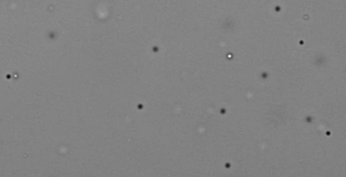
’’…observe whenever the rays are let in and pour the sunlight through the dark chambers of houses: , and as in never-ending conflict skirmish and give battle combating in troops and never halting, driven about in frequent meetings and partings; so that you may guess from this, what it is for first-beginnings of things to be ever tossing about in the great void. So far as it goes, a small thing may give an illustration of great things and put you on the track of knowledge. And for this reason too it is meet that you should give greater heed to these bodies which are seen to tumble about in the sun’s rays, . All you are to know derive this restlessness from the first-beginnings. For the first-beginnings of things move first of themselves; next those bodies which form a small aggregate and come nearest so to say to the powers of the first-beginnings, are impelled and , and they next in turn stir up bodies which are a little larger. .

– ‘Nature of Things’ (circa 60 BC) by¹

Important

Please be careful, handle the microscope and lenses carefully — they are precision instruments.
Never force knobs or adjustments. If something feels stuck, ask for help.

Introduction

The atoms and molecules that make up matter are in constant random motion. This microscopic agitation is the thermal kinetic energy that we interpret as temperature. A direct consequence of this ceaseless jostling is that larger particles suspended in a fluid display an erratic, zig-zag motion. This phenomenon, now called Brownian motion, was first observed by the botanist Robert Brown in 1827 (though Lucretius had already imagined such motions long before).

Brownian motion is of fundamental importance because it provided some of the earliest convincing evidence for the atomic nature of matter. In this project, you will observe Brownian motion using an optical microscope and connect what you see to the models developed by Einstein, Langevin, and others.

In 1905, Einstein presented a mathematical model to explain Brownian motion².¹ His work was soon followed by Smoluchowski in 1906 and by Langevin in 1908⁴. In the same year, Jean Perrin performed careful measurements to test Einstein’s predictions and to make the first experimental estimate of the Boltzmann constant $k_B$. Perrin received the 1926 Nobel Prize in Physics for this achievement. Sadly, Boltzmann himself had already passed away by then.

In this project, you will observe Brownian motion and collect data to estimate the Boltzmann constant. You will adopt Langevin’s approach² to understand the theory of Brownian motion.

Project Details

Your PI has recently purchased new equipment to begin a series of diffusion experiments aimed at studying molecular interactions.
To get started, she needs your help setting up the system and establishing reliable protocols for using the imaging setup to make quantitative measurements.

The simplest experiment she can think of to begin with is measuring the Boltzmann constant ($k_B$) through observations of Brownian motion.
Your task is to help her design, build, and test this experiment on the Nikon LV100D microscope system.

By the end of this project, you should be able to:

Operate and optimise new instruments and software.
Use the Nikon LV100D microscope, NIS Elements, and ImageJ effectively.
Design and refine an experiment.
Build a DIY sample chamber, prepare bead suspensions, and optimise observation conditions.
Quantify uncertainties.
Identify sources of error and propagate uncertainties to assess the robustness of your $k_B$ estimate.
Connect theory to observation.
- Relate measured mean-square displacements to the Langevin/Einstien framework and interpret results.
- Relate relevant optical concepts to experiments.

By the end of this exercise you will have to have:

Operational knowledge of the LV100D microscope (demonstrated during discussion/viva).
A short video recording of Brownian motion of microbeads.
Tracked position data (from ImageJ or Python) for selected particles.
An estimate of $k_B$ derived from your analysis (with working).
An error analysis explaining uncertainties, assumptions, and limitations of your approach.

Start early: sample prep and alignment often take longer than expected.
Work iteratively: make one change at a time, observe, and refine.
Share the load: e.g., sample prep, imaging, trackin, Python analysis.
Keep a group logbook: record dates, plans, attempts, what worked/didn’t, and next steps; this supports grading and your own learning.

Equipment & Resources

Optical Microscope (Nikon Eclipse LV100D) with camera and image-capturing software.
Microspheres
Dr Robert has kindly prepared a sample of 50 μm microspheres (Bang’s Labs, lot #5855, Inv #L030620C), supplied as a 10.2% (w/v) solution. You will need to prepare a sample chamber to work with these beads.
- Mix the bead suspension
  Vortex for 10–15 seconds or sonicate briefly in a water bath.
- Prepare dilutions using serial dilution in deionized water.
  These dilutions can be stored at 4 °C for up to ~1 week.
  
  Example (8.31 μm beads, label “B”):
  - Step 1: Mix 3 μL beads + 297 μL water → 1:100 dilution.
  - Step 2: Take 100 μL from Step 1 + 900 μL water → 1:10 dilution.
  - Final dilution = 1:1000.
DIY Chamber
You can prepare 2-chamber slides in either of two ways:
- Using double-sided tape between the coverslip and glass slide, or
- By gently heating parafilm between the coverslip and slide.

ImageJ2
MosaicSuite plugin for ImageJ
NIS Elements – already installed on the computers in the Dry Lab.

ECLIPSE LV100D
LV-UEPI Instructions

The Microscope

The Nikon ECLIPSE LV100D

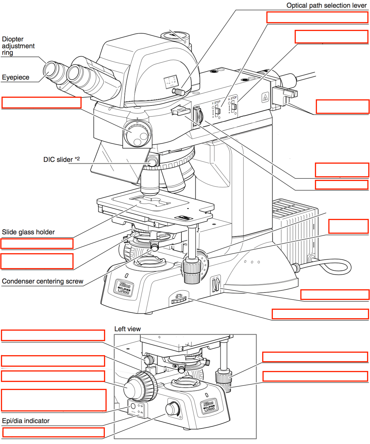
One of your first task is to get familiar with the ECLIPSE LV100D Nikon upright microscope. For this:

Use Figure 1 to identify the various components (buttons, knobs, levers, sliders, etc.) of the microscope.
Identify what each of the listed items is meant for and whether it is relevant for your experiment.
Note the precautions you should take when using each component.
Fill in Table 1 to ensure you understand what each is meant to do.

Item	What does it do?	Do you need it?	Precautions
Bright Field Microscopy
Dark Field Microscopy
Fluorescence Microscopy
Episcopic illumination
Diascopic illumination
Aperture diaphragm
Field diaphragm
Condenser
Condenser Aperture diaphragm
Objective
Filter Slides
Focus knobs			Do not over-rotate. Do not counter-rotate left and right knobs.
ND Filters
NCB Filters

Table 1: Important Microscope related components and terms

Figure 1: Important Microscope components.

A Word About Optics

This experiment is about optimising your sample and optical setup to obtain the highest-quality images possible. Take time to adjust the microscope, refine the illumination, and check that the image quality is uniform across the field of view.

Your goal is to capture images from which you can accurately extract positional information. To do this, you need to understand a few key optical concepts; particularly resolution, the point spread function (PSF), and the numerical aperture (NA). These determine how precisely you can locate and distinguish the beads you are tracking, both laterally and axially. For this you will need to appreciate how microscopes are diffraction limited instruments.

Illumination is also an important factor. Variations in brightness or focus can affect the accuracy of particle tracking and introduce systematic errors. Proper Köhler illumination and stable focus are therefore essential for reliable measurements.

Remember to explore the different imaging modes available on the microscope. Each mode (brightfield, darkfield, or phase contrast) reveals different features of the same sample and can help you find the best conditions for visualising Brownian motion.

Finally, don’t forget about calibration and the impact of your digital imaging setup on issues such as motion blur, pixel scaling errors, and timing inaccuracies.

Langevin’s Theory of Brownian Motion

A Quick Summary

Brownian motion is an example of the statistical fluctuations that occur in a system at thermal equilibrium. In 1905, Einstein² presented a mathematical model to explain Brownian motion.³ This was followed by a treatment by Smoluchowski in 1906 and Langevin⁴ in 1908. In this project we will use Langevin’s approach, which is often described as “infinitely more simple” than Einstein’s.

Figure 2: Trajectories of several microbeads.

According to Langevin’s theory the relationship between time, $t$, and the mean square of the distance moved, $\ex{R_t^2}$, is given by

\[ \ex{R_t^{2}} = \ex{x_t^{2}}+ \ex{y_t^{2}}= \frac{2 k_{B}T}{3 \pi \eta a}t \tag{1}\]

$T$ is the temperature, $\eta$ the viscosity of medium (water in this case) and $a$ the radius of the spheres.

Langevin’s Theory Expanded

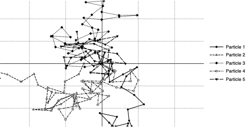
In Brownian motion, the Brownian particle is constantly bombarded by the molecules that make up the medium. These bombardments are extraordinarily frequent; about $10^{14}$ per second(!). The zig-zag paths we observe (see Figure 2) represent the averaged effect of these countless collisions.

Our goal is to quantify the motion of Brownian particles. Specifically, we want to know how far, on average, a particle moves from its starting point after a given time or a certain number of steps.

What parameter?

What parameter should we use to measure this? A quick look at Figure 2 shows that the various paths have no preferred direction. If we find a particle at position $(x_{t}, y_{t}, z_{t})$ at time $t$, it is just as likely that another particle will be found at $(-x_{t}, -y_{t}, -z_{t})$. Thus, when we average over a large number of identical particles (called ensemble average), the mean displacement in each direction is zero:
\[ \langle x_{t} \rangle \;=\; \langle y_{t} \rangle \;=\; \langle z_{t} \rangle \;=\; 0 \tag{2}\]

A more suitable quantity to describe how far the particles end up from their starting point are the mean-square displacements: $\langle x_{t}^{2} \rangle$, $\langle y_{t}^{2} \rangle$, and $\langle z_{t}^{2} \rangle$. More specifically, if $R_{t}$ is the distance of the particle from the starting point after a time $t$, then

\[ \langle R_{t}^{2} \rangle = \langle x_{t}^{2} \rangle + \langle y_{t}^{2} \rangle + \langle z_{t}^{2} \rangle \tag{3}\]

If we were to consider a general system, there is nothing special about the $x$, $y$, or $z$ directions, we expect symmetry in the averages:
\[ \langle x_{t}^{2} \rangle = \langle y_{t}^{2} \rangle = \langle z_{t}^{2} \rangle \]

Hence,

\[ \ex{R_{t}^{2}} = \left\{\begin{array}{rcr} \ex{x_{t}^{2}} & & \text{For $1$D} \\ 2\,\ex{x_{t}^{2}} & & \text{For $2$D} \\ 3\,\ex{x_{t}^{2}} & & \text{For $3$D} \end{array}\right. \tag{4}\]

Lets proceed first by working in 1D (the $x$ direction). We can later extend to two or three dimensions using equation Equation 4. The following analysis is based on material from⁵,⁶,⁷ and⁸.

A General Particle Moving in a Fluid

To determine $\langle x_{t}^{2} \rangle$ for the Brownian particle, we first need to understand how a particle moves through a fluid.
One of the key effects we must consider is the resistive drag force, which is described by Stokes’ Law.

Stokes’ Law

The viscous (drag) resistive force experienced by a sphere of radius $a$ moving through a fluid at speed $v$ is given by

\[ F_{\text{drag}} = 6\pi \eta a v \tag{5}\]

where $\eta$ is the coefficient of viscosity, which characterises how easy or hard it is to move through the fluid.

To continue with our analysis, consider a spherical particle of mass $m$ moving through a fluid in the $x$-direction under the action of a time-dependent force $F_{x}(t)$.

Applying Newton’s Second Law, we can write the equation of motion as:

\[ m \frac{dv}{dt} = -6\pi \eta a\, v + F_{x}(t) \tag{2} \]

Lets recast, this relationship in terms of only $x$ and $t$ by using the fact that $v=\da{x}{t}$: \[ m\daa{x}{t}=- \alpha \, \da{x}{t} + F_{x}(t) \tag{6}\]

We have used $\alpha=6\pi \eta a$ for convenience.

A Brownian Particle Moving in a Fluid

A Brownian particle experiences numerous bombardments in a given time $t$. Our task is to figure out what resulting movement (specifically $\ex{x^{2}}$) such bombardments will cause. Lets start by using Equation 6 in the context of Brownian motion.

Lets start by multiplying by $x$ to yield:

\[ mx\daa{x}{t}=- \alpha\, x\da{x}{t} + xF_{x} \tag{7}\]

Notice that:

\[ \begin{align*} \da{}{t}\lr{x\da{x}{t}}&=\lr{\da{x}{t}}^{2}+x\daa{x}{t} \\ \Rightarrow x\daa{x}{t} &= \da{}{t} \lr{x\da{x}{t}}-\lr{\da{x}{t}}^{2} \end{align*} \tag{8}\]

therefore,

\[ % \begin{subequations} \begin{align} \Rightarrow\quad m\lrs{\da{}{t} \lr{x\da{x}{t}}-\lr{\da{x}{t}}^{2}}&=- \alpha\, x\da{x}{t} + xF_{x}\\ \text{i.e.}\quad m\lrs{\da{}{t} \lr{xv}-{v}^{2}}&=- \alpha\, (xv) + xF_{x}\\[1em] \text{i.e.}\quad m\da{}{t} \lr{xv}-m{v}^{2}&=- \alpha\, (xv) + xF_{x}\label{equ:oneParticle} \end{align} % \end{subequations} \tag{9}\]

An Ensemble of Brownian Particles Moving in a Fluid

Now lets consider an ensemble of Brownian particles. The motion of each of these particles will be described by an equation such as Equation 9. I.e. if we have a $N$ s, will have $N$ such equations.
\[ \renewcommand{\temp}[1]{ m\da{}{t} \lr{x_{#1}v_{#1}}-m{v_{#1}}^{2}&=- \alpha\, (x_{#1}v_{#1}) + x_{#1}\,F_{x_{#1}}(t) } \begin{align*} \temp{1}\\ \temp{2}\\ \temp{3}\\ \ldots\ldots & \ldots\ldots\\ \temp{N}\\ \end{align*} \] If we take the average of all these equations we get:

\[ m\da{}{t} \ex{xv}-2\ex{\frac{1}{2} m{v}^{2}}=- \alpha\, \ex{xv} + \ex{xF_{x}(t)} \tag{10}\]

Let’s try to simplify this equation a bit.

$F_{x}(t)$ is a time-dependent force representing the random kicks given by the thermal motion of the fluid molecules. There is no dependence (correlation) between $x$ and $F_{x}$ — meaning that the kick a particle receives does not depend on its position. As a result, the ensemble average of their product becomes zero.

To see why, note that the ensemble averages of $x$ and $F_x$ can be written as:

\[ \begin{align} \langle x \rangle &= \sum_i p_i^{(x)}\, x_i \\ \langle F_x \rangle &= \sum_j p_j^{(F)}\, F_j \end{align} \]

Here, $p_i^{(x)}$ and $j^{(F)}$ denote the probabilities of obtaining the values $x_i$ and $F_j$, respectively.

Since $x$ and $F_x$ are uncorrelated and independent, the joint probability of obtaining both $x_i$ and $F_j$ is simply the product of their individual probabilities: \[ p_{ij}^{(x,F)} = p_i^{(x)} \, p_j^{(F)}. \]

Hence, \[ \langle x F_x(t) \rangle = \sum_i \sum_j p_i^{(x)} p_j^{(F)} \, x_i F_j = \left( \sum_i p_i^{(x)} x_i \right) \left( \sum_j p_j^{(F)} F_j \right) = \langle x \rangle \, \langle F_x(t) \rangle \] However, since $F_x(t)$ represents a random ‘kick’, its ensemble average must be zero. I.e. on average, the random forces do not favour any direction. Hence,
\[ \langle x F_x(t) \rangle = 0 \]

This simplifies Equation 10 to:

\[ m\da{}{t} \ex{xv}-2\ex{\frac{1}{2} m{v}^{2}}=- \alpha\, \ex{xv} \tag{11}\]

Let’s assume that the Brownian particle is in thermal equilibrium with the surrounding fluid, and therefore with the same temperature. Recall the the definition of temperature, that relates it to the the average kinetic energy of the particles, allowing us to write: \[ \text{average KE}= \left\langle \frac{1}{2} m v^{2} \right\rangle = \frac{1}{2} k_{B} T \tag{12}\]

Note that this is for a particle moving in one dimension.

Equation 11 now looks:

\[ m\da{}{t} \ex{xv}-k_{B} T=- \alpha\, \ex{xv} \tag{13}\]

This is a differential equation in $\ex{xv}$ can readily be solved (see Section 5.3) to get:

\[ \ex{xv} = \frac{k_{B}T}{\alpha} -e^{\displaystyle\lr{-\f{\alpha}{m} t+C_{1}}} \]

If take that all the particles start at $x=0$, $\ex{xv}=0$ at $t=0$.

This means \[ 0 = \frac{k_{B}T}{\alpha} -e^{C_{1}} \Rightarrow e^{C_{1}} =\frac{k_{B}T}{\alpha} \]

Whence, \[ \ex{xv} = \frac{k_{B}T}{\alpha}\lrs{1-e^{\displaystyle-\frac{\alpha}{m} t}} \]

This shows that $\ex{xv}$ tends to the value $\displaystyle \frac{k_{B}T}{\alpha}$ at time goes by.

For the time scales we are interested in, we can take this to occur instantaneously, so that:

\[ \ex{xv} = \frac{k_{B}T}{\alpha} \tag{14}\]

Now we need a way to tease out $\ex{x^2}$ from Equation 14. For this note that:

\[ \begin{align} \da{x^{2}}{t} &= 2x\lr{\da{x}{t}}=2(xv) \\ \Rightarrow\da{}{t}\ex{x^{2}} &= 2\ex{xv}\\ \end{align} \]

Using this with Equation 14: \[\begin{align*} \da{}{t}\ex{x^{2}}&= \frac{2 k_{B}T}{\alpha}\\ \Rightarrow \ex{x^{2}} &= \frac{2 k_{B}T}{\alpha}t + C_{2} \end{align*}\] Since, $x=0$ at $t=0$, $C_{2}=0$:

\[ \ex{x^{2}} = \frac{2 k_{B}T}{\alpha}t = \frac{ k_{B}T}{3 \pi \eta a}t \]

Finally(!), using equations Equation 3 and Equation 4, for a 2D situation, we can write: \[ \ex{R^{2}} = \ex{x^{2}}+ \ex{y^{2}}= \frac{2 k_{B}T}{3 \pi \eta a}t \tag{15}\]

Sometimes, you will encounter this relationship in the form:

\[ \ex{R^{2}} = 2 n D t \tag{16}\]

Where, $n$ is the dimensionality of the motion⁴ and

\[ D= \frac{k_{B}T}{6 \pi \eta a} \]

is called the Diffusion constant.

Appendix: Solving differential equation

To solve the differential equation lets use the following substitution

\[ y\equiv k_{B}T-\alpha\ex{xv} \Rightarrow \da{y}{t}=-\alpha\da{}{t}\ex{xv} \]

This will convert equation Equation 13 into:

\[ \begin{align*} m\da{y}{t}&=\alpha y\\ \Rightarrow \da{y}{t}&=-\frac{\alpha}{m} y\\ \Rightarrow \int\frac{1}{y} dy &=- \frac{\alpha}{m} \int dt + C_{1}\\ \Rightarrow \ln y &=- \frac{\alpha}{m} t+C_{1}\\ \Rightarrow k_{B}T-\alpha\ex{xv} &=e^{-\displaystyle \frac{\alpha}{m} t+C_{1}}\\ \text{i.e.}\quad \ex{xv} &= \frac{k_{B}T}{\alpha} -e^{-\displaystyle \frac{\alpha}{m} t+C_{1}} \end{align*} \]

Chapter References

Lucretius Carus, T. On the Nature of Things. (Hackett Publishing, Indianapolis, IN, 2001).

Einstein, A. On the motion of small particles suspended in a stationary liquid, as required by the molecular kinetic theory of heat. Annalen der Physik 322, 549–560 (1905).

Bernstein, J. Einstein and the existence of atoms. American Journal of Physics 74, 863–872 (2006).

Lemons, D. S. Paul langevin’s 1908 paper "on the theory of brownian motion". American Journal of Physics 65, 1079 (1997).

Berg, H. C. Random Walks in Biology. (Princeton University Press, Princeton, NJ, 1993).

Reif, F. Fundamentals of Statistical and Thermal Physics. (McGraw-Hill, New York, 1965).

Denny, M. W. & Gaines, S. Chance in Biology: Using Probability to Explore Nature. (Princeton University Press, Princeton, NJ, 2000).

Nakroshis, P., Amoroso, M., Legere, J. & Smith, C. Measuring boltzmann’s constant using video microscopy of brownian motion. American Journal of Physics 71, 568 (2003).

Footnotes

Einstein was apparently unaware of Robert Brown’s earlier observations³.↩︎
often described as “infinitely more simple” than Einstein’s↩︎
Einstein was apparently unaware of Robert Brown’s earlier observations³.↩︎
2 in the case of Equation 15 ↩︎