Basic Ideas

Activity 1 | Week 2 | Background

What to expect

In this chapter, I introduce the basic physics and mathematics we need to understand how a simple pendulum moves and, eventually, to build a mathematical model of it. These ideas are fundamental, and you will find them useful even beyond 76.

1 Calculus

Science largely involves system that change: we change one quantity, observe what happens to another, and try to explain and predict the result. Calculus is the language we use to describe this change.

When I say calculus, you might immediately think of expressions like:

\[ \frac{d}{dx}x^2=2x \tag{1}\]

\[ \int x\,dx=\frac{1}{2}x^2+C. \tag{2}\]

This is the mechanical side of calculus, and software (e.g., SymPy, Maple, Mathematica, Wolfram Alpha) can often work them out for us. What matters for 76 is understanding what calculus means and how it helps us describe a changing system.

1.1 Differentiation

The derivative shown below It tells us how much \(y\) will change if we change \(x\) by one unit. I.e. it tells us the rate of change of \(y\) with respect to \(x\).

\[ \frac{dy}{dx} \tag{3}\]

Sometimes it is easier to find meaning in such an equation by thinking of it as a fractions:

The meaning of differentiation

\[ \dfrac{dy}{dx}\approx \dfrac{\Delta y}{\Delta x} \qquad\Rightarrow\qquad \Delta y \approx \lr{\dfrac{dy}{dx}}\Delta x \tag{4}\]

The approximation gets better, the smaller you make \(\Delta x\).

For example, consider

\[ \frac{dN}{dt}=-\lambda N. \tag{5}\]

Over a small time step \(\Delta t\),

\[ \Delta N\approx-\lambda N\Delta t. \tag{6}\]

This tells us two things immediately:

\(N\) decreases because the rate is negative
the larger \(N\) is, the faster it decreases

With practice, you will learn to read this story directly from Equation 10.

1.2 Integration

One way to understand

\[ \int_a^b f(x)\,dx \tag{7}\]

is as the area under the curve \(f(x)\). The central idea is simple: split the area into thin rectangles and add them.

More formally,

\[ \int_a^b f(x)\,dx \approx \sum_{i=1}^{n} f(x_i^*)\Delta x_i. \tag{8}\]

Here, \(\Delta x_i\) is the width of a slice and \(f(x_i^*)\) is its height. Their product is the area of one rectangle. Adding all the rectangles approximates the integral.

As the slices become increasingly narrow, the approximation approaches the exact result:

The meaning of integration

\[ \int_a^b f(x)\,dx = \lim_{\max_i(\Delta x_i)\to 0} \sum_{i=1}^{n} f(x_i^*)\Delta x_i. \tag{9}\]

This is why integration is a process of summation.

Figure 1: Riemann sum for \(y=x^2\) over \([0,2]\).
(Source: Wikipedia)

1.3 Solving differential equations

We often model changing systems using differential equations, such as

\[ \frac{dN}{dt}=-\lambda N. \tag{10}\]

The hardest part is usually constructing the equation. This requires us to understand the underlying science and express it using calculus.

A solution tells us explicitly how the system changes. If we are lucky, a little mathematical wizardry gives us an exact analytical solution. For Equation 10,

\[ N(t)=N_0e^{-\lambda t}, \]

where \(N_0\) is the value of \(N\) at \(t=0\).

Many realistic differential equations do not have a useful analytical solution. This is where numerical methods come in.

Euler’s method, which you encountered previously in 73, uses Equation 4 to approximate the evolution of a system one small step at a time.

1.4 Higher-order derivatives

We often need the rate of change of a rate of change. For example,

\[ \da{}{x}\lr{\da{y}{x}}. \tag{11}\]

This is the second derivative of \(y\) with respect to \(x\), written as

\[ \da{}{x}\lr{\da{y}{x}}=\daa{y}{x}. \tag{12}\]

A relevant example is motion (see Section 2.3): velocity is the rate of change of position, while acceleration is the rate of change of velocity.

2 Vectors & Scalars

Physical quantities can be either scalars or vectors.

Scalar A scalar has only a size(magnitude).
Examples include mass (\(50\,\mathrm{kg}\)), temperature (\(-20\,^\circ\mathrm{C}\)), and distance (\(100\,\mathrm{km}\)).

Vector A vector has both a magnitude and a direction.
Examples include a force of \(10\,\mathrm{N}\) downwards and a velocity of \(50\,\mathrm{km\,h^{-1}}\) north.

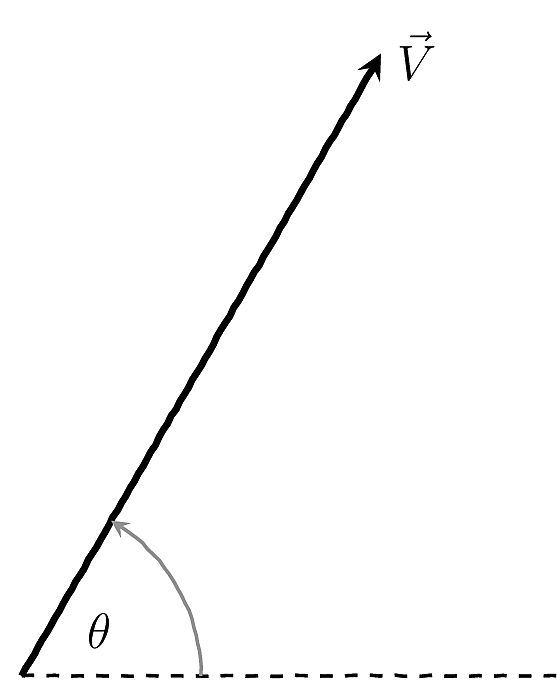
We represent vectors using an arrow, such as \(\vec{X}\), or a bold symbol, \(\mathbf{X}\). The arrow’s direction and length represent the vector’s direction and magnitude as seen in Figure 3.

2.1 Components & Resultant Of A Vector

Adding and subtracting vectors is interesting because we must take direction into account. Two key ideas here are the resultant and components.

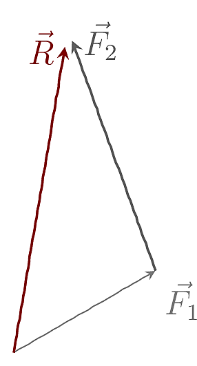
Resultant As shown in Figure 4, two vectors can be combined (added) to give a single vector. This is called the resultant, and it has the same overall effect as the original vectors combined. The standard way to add vectors is to draw them end to end.

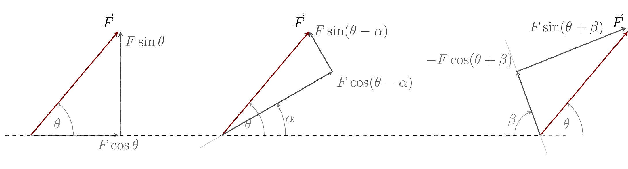
Components Just as we can combine vectors to form one, we can also reverse the process and split a vector into parts, called its components. Figure 2 shows three ways of splitting one vector (\(\vec{F}\), shown in colour) into two others¹. The most common and useful choice is to split into two perpendicular directions (leftmost).

Figure 2: Three ways the same vector (shown in **colour**) is split into components.

Figure 3: A vector has a size and a direction.

Figure 4: Two or more vectors can be added to give a single resultant vector. In this example the resultant \(\vec{R}\) produces the same effect as the combination of vectors \(\vec{F}_1\) and \(\vec{F}_2\).

Perpendicular components

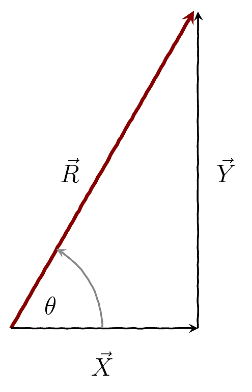
One very convenient way to split a vector is into two (or three, in 3D) perpendicular components. We can then use Pythagoras’ theorem to reconstruct the resultant.

For the components shown in Figure 5, the magnitude of the resultant is \[ |\vec{R}| = R = \sqrt{X^2 + Y^2}, \tag{13}\]

and its direction, measured from the positive \(x\)-axis, satisfies

\[ \tan\theta = \dfrac{Y}{X}. \tag{14}\]

For three perpendicular components,

\[ |\vec{R}| = R = \sqrt{X^2 + Y^2 + Z^2}. \tag{15}\]

Figure 5: Resultant of two perpendicular vectors.

2.2 Play with vectors

You can try out the ideas above using the following applet (from ).
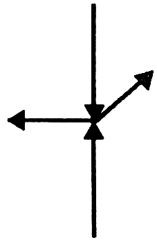
For instance Use the applet (Lab) to find the resultant of the set of vectors shown in the adjoining figure.

2.3 Speed, Velocity and Acceleration

Speed, velocity, and acceleration are three quantities we need to understand the motion of a pendulum. Each has a linear form for straight-line motion and an angular form for rotational motion.

Linear motion

Speed (\(\mathrm{m\,s^{-1}}\)) tells us how fast an object is moving. It is a scalar.

\[ v=\da{x}{t} \tag{16}\]

Velocity (\(\mathrm{m\,s^{-1}}\)) tells us how fast and in which direction the object is moving.

\[ \vec{v}=\da{\vec{x}}{t} \tag{17}\]

Acceleration (\(\mathrm{m\,s^{-2}}\)) tells us how quickly the velocity is changing.

\[ \vec{a} =\da{\vec{v}}{t} =\daa{\vec{x}}{t} \tag{18}\]

I am sure you are familiar with:

\[ \text{average speed} = \frac{\text{total distance}}{\text{elapsed time}}. \tag{19}\]

This gives the speed over a time interval. Equation 16 expresses the same idea but for a very small time interval, giving the speed at a particular instant, making it more useful for modelling a changing system.

Angular motion

Angular motion describes movement around a circular path of radius \(r\).

We use:

\(\theta\) for angular position,
\(\omega\) for angular velocity, and
\(\alpha\) for angular acceleration.

If the object moves through an angle \(\theta\) (measured in radians) the distance travelled along the circular path is

\[ s=r\theta. \tag{20}\]

For a constant radius, differentiating with respect to time gives the tangential speed:

\[ v=\da{s}{t} =r\da{\theta}{t} =r\omega. \tag{21}\]

Figure 6: Various parameters related to angular motion.

Differentiating again gives the tangential acceleration:

\[ a_{\mathrm{t}} =\da{v}{t} =r\da{\omega}{t} =r\alpha. \tag{22}\]

An object moving in a circle also has an acceleration directed towards the centre called, centripetal acceleration:

\[ a_{\mathrm{r}}=\frac{v^2}{r}=r\omega^2. \tag{23}\]

3 Forces

3.1 What is a force?

A force is a push or a pull.

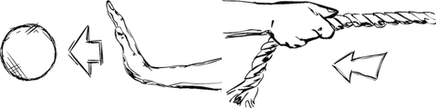
Force is a vector, so it has both magnitude and direction. As shown in Figure 8, a net force changes the velocity of a mass: it can change its speed, its direction, or both.

The SI unit of force is the newton (\(\mathrm{N}\))².

3.2 Newton’s laws

Newton’s three laws form the foundation of classical mechanics:

The first law tells us that changing an object’s velocity requires a net force.
The second law, quantifies that change: \[ \vec{F}_{\mathrm{net}}=m\vec{a} \tag{24}\]
The third law tells us that forces arise through interactions: two objects exert equal-but-opposite forces on each other.

For the pendulum, we will mainly use Newton’s second law.

Figure 8: A net force changes the velocity of a mass.

4 Simple harmonic motion (SHM)

I am going to kill two birds with one stone: show you how to use Python to do calculus and introduce you to a special type of motion.

Simple harmonic motion (SHM) appears almost everywhere: vibrating guitar strings, atomic vibrations, swaying branches, springs… . Physicists have therefore studied it extensively.

You are already familiar with this motion. Imagine a box attached to a spring. Pull the box and the spring pulls it back. Push the box and the spring pushes it out. The further you move the box, the stronger this restoring force becomes:

\[ F=-kx, \tag{25}\]

where \(x\) is the displacement from equilibrium (where there is no force) and \(k\) describes the stiffness of the spring. The negative sign tells us that the force always points towards equilibrium.

A horizontal spring-mass system oscillating about the origin with an amplitude \(A\) (Source here)

Using Newton’s second law (Equation 24),

\[ \begin{align} F &= ma\\ \text{i.e.}\quad-kx &= m\daa{x}{t} \end{align} \tag{26}\]

Rearranging,

\[ \daa{x}{t}+\frac{k}{m}x=0. \]

We can make this look nicer and more intuitive by defining,

\[ \omega^2=\frac{k}{m}, \tag{27}\]

so that equation becomes

\[ \daa{x}{t}=-\omega^2x. \tag{28}\]

A solution to Equation 28 is

\[ x(t)=A\sin(\omega t)+B\cos(\omega t), \tag{29}\]

where \(A\) and \(B\) are constants that depend on how the motion begins.

Let us verify this using SymPy (please visit the SPS Python Website for more examples):

import sympy as sp

t = sp.symbols("t", real=True)
A, B, omega = sp.symbols("A B omega", real=True)

x = A * sp.sin(omega * t) + B * sp.cos(omega * t)

# Differentiate once to obtain velocity
velocity = sp.diff(x, t)

# Differentiate twice to obtain acceleration
acceleration = sp.diff(x, t, 2)

print('velocity: ', velocity)
## velocity:  A*omega*cos(omega*t) - B*omega*sin(omega*t)
print('acceleration: ', acceleration)
## acceleration:  -omega**2*(A*sin(omega*t) + B*cos(omega*t))

Let me display the acceleration in a prettier form so that the result is easier to recognise:

\[- \omega^{2} \left(A \sin{\left(\omega t \right)} + B \cos{\left(\omega t \right)}\right)\]

The expression in parentheses is \(x(t)\), so SymPy has shown that

\[ \daa{x}{t}=-\omega^2x, \] which is precisely Equation 28 for simple harmonic motion!

5 Energy

Let me briefly introduce energy.

5.1 Forms of energy

The three forms that interest us most are:

Kinetic energy, the energy associated with motion: \[ \text{KE}=\frac{1}{2}mv^2, \tag{30}\]

where \(m\) is the mass and \(v\) is its speed.
Gravitational potential energy, the energy associated with position in a gravitational field: \[ \text{GPE}=mgh, \tag{31}\]

where \(g\) is the acceleration due to gravity and \(h\) is the height above a chosen reference point.
Elastic potential energy, the energy stored when a spring is stretched or compressed: \[ \text{EPE}=\frac{1}{2}kx^2, \tag{32}\]

where \(k\) is the spring constant and \(x\) is the displacement from equilibrium.

5.2 Energy is conserved

Energy can move between these forms, but the total energy of an isolated system is conserved:

Energy cannot be created or destroyed, only transferred or transformed.

For an ideal pendulum, energy continually changes between kinetic and gravitational potential energy while their sum remains constant. This gives us a powerful way to check whether our computational model behaves sensibly.

6 Useful Approximations

6.1 Taylor Series

I would like to wrap up this chapter by introducing you to a simple idea that will help you in many different situations. It is called the Taylor series expansion, and it allows you to think of a function as a series of powers.

More formally, the Taylor series of a function \(f(x)\) around a point \(x = x_0\) is defined as:

\[ f(x) = f(x_0) + f'(x_0)(x - x_0) + \frac{f''(x_0)}{2!}(x - x_0)^2 + \frac{f^{(3)}(x_0)}{3!}(x - x_0)^3 + \cdots \]

It is important to keep in mind that this is an approximation that is built around a specific point: \(x = x_0\). The farther you move away from this point, the less accurate the approximation becomes. How far is “too far” depends on the function you are working with.

6.2 Maclaurin Series

Here are the Taylor series for some commonly used functions around \(x = 0\). This special case where the expansion is about zero is called the Maclaurin series.

\[ e^x = 1 + x + \frac{x^2}{2!} + \frac{x^3}{3!} + \cdots \tag{33}\]

\[ \sin x = x - \frac{x^3}{3!} + \frac{x^5}{5!} - \frac{x^7}{7!} + \cdots \tag{34}\]

\[ \cos x = 1 - \frac{x^2}{2!} + \frac{x^4}{4!} - \frac{x^6}{6!} + \cdots \tag{35}\]

\[ \tan x = x + \frac{x^3}{3} + \frac{2x^5}{15} + \frac{17x^7}{315} + \cdots \tag{36}\]

Footnotes

A vector can be split into more than two components, but this is usually unnecessary.↩︎
Approximately the weight of a typical apple.↩︎