flowchart LR
    A["Measure<br/>T₁₀ and T₂₀"]
    B["Look for a<br/>difference"]
    C["Construct a<br/>physical model"]
    D["Small-angle<br/>approximation"]
    E["Numerical<br/>model"]
    F["Forward Euler<br/>(simple, but unstable)"]
    G["Euler–Cromer<br/>(better behaved)"]

    A --> B --> C
    C --> D
    C --> E
    E --> F --> G

    classDef experiment fill:#e8f1fb,stroke:#27628a,stroke-width:2px,color:#111;
    classDef theory fill:#f5ead7,stroke:#a26721,stroke-width:2px,color:#111;
    classDef computation fill:#e5f3e7,stroke:#347a3d,stroke-width:2px,color:#111;

    class A,B experiment;
    class C,D theory;
    class E,F,G computation;
Asking difficult questions with a numerical model
Activity 1 | Week 3 | IS
\[ % \newcommand\v[1]{\vec{#1}} % \newcommand\v[1]{\mathbf{#1}} \newcommand\v[1]{\boldsymbol{#1}} \newcommand\vdot[2]{\v{#1}\cdot\v{#2}} \]
\[ \newcommand{\dd}[2][]{\mathrm{d}^{#1}#2} \]
\[ \newcommand\f[2]{\dfrac{#1}{#2}} \newcommand\da[2]{\dfrac{d #1}{d #2}} \newcommand\daa[2]{\dfrac{d^2 #1}{d #2^2}} \newcommand\pa[2]{\dfrac{\partial #1}{\partial #2}} \newcommand\paa[2]{\dfrac{\partial^2 #1}{\partial #2^2}} \newcommand\pab[3]{\dfrac{\partial^2 #1}{\partial #2 \partial #3}} \def\half{\frac{1}{2}} \]
\[ \newcommand\ket[1]{\left|#1\right\rangle} % |x> \newcommand\exp[1]{\left\langle#1\right\rangle} % <x> \newcommand\lr[1]{\left(#1\right)} % (x) \newcommand\lrs[1]{\left[#1\right]} % [x] %\newcommand\lrb[1]{\left|#1\right|} % |x| \newcommand\lra[1]{\left|#1\right|} % |x| \newcommand\lrc[1]{\left\{#1\right\}} % {x} \newcommand\lrl[3]{\left.#1\right|_{#2}^{#3}} % x_limits \]
\[ \def\ie{\text{i.e.}\quad} \]
$$ % Typical reaction % Nuclear reactions
$$
\[ \newcommand{\coulomb}[1]{\dfrac{#1}{4\pi\epsilon_0}} \]
\[ \def\amu{\text{ amu}} \def\J{\text{ J}} \def\K{\text{ K}} \def\s{\text{ s}} \def\second{\text{ s}} \def\Psecond{\text{ s}^{-1}} \def\m{\text{ m}} \def\mm{\text{ mm}} \def\km{\text{ km}} \def\fm{\text{ fm}} \def\mum{\text{ $\mu$m}} \def\mus{\text{ $\mu$s}} \def\mPERs{\text{ ms$^{-1}$}} \def\eV{\text{ eV}} \def\keV{\text{ keV}} \def\GeV{\text{ GeV}} \def\MeV{\text{ MeV}} \def\MeVc{\text{ MeV/c$^2$}} \def\KeVc{\text{ KeV/c$^2$}} \newcommand\ttp[1]{\times 10^{#1}} % To The Power \]
$$
$$
\[ \def\uraniumA{_{92}^{233}{\text{U}}_{}} \def\uraniumB{_{92}^{235}{\text{U}}_{}} \def\uraniumC{_{92}^{238}{\text{U}}_{}} \def\carbonB{_{6}^{14}{\text{C}}_{}} \def\nitrogenB{_{7}^{14}{\text{N}}_{}} \def\oxygenA{_{8}^{14}{\text{O}}_{}} \def\oxygenB{_{8}^{16}{\text{O}}_{}} \]
\[ \def\com{\text{\scriptsize CM}} \]
\[ \def\l{\ell} \def\l{l} \]
\[ \def\g{\gamma} \def\g{\gamma} \]
1 What to expect
So far, we have developed a model of the simple pendulum and solved it using both the small-angle approximation and numerical integration. Our investigative journey is summarised in Figure 1.
What we have done helps us understand the difference between \(T_{10^\circ}\) and \(T_{20^\circ}\). However, the model has not yet given us much insight into how we could improve the experiment.
That is what I want to focus on today. I want us to make the model more realistic, compare it with evidence, and then use it to investigate questions that would be difficult to isolate experimentally.
This is one of the most powerful uses of computation in science. A model allows us to explore situations beyond our immediate experimental reach. For example:
- AlphaFold predicts three-dimensional protein structures
- SRIM models how ions travel through matter
- CASINO simulates electron trajectories in solids
- Spartan predicts molecular structures and properties
- COMSOL
These models do not replace experiments. They help us decide what to expect, what to measure, and which experiments are worth doing.
1.1 The questions
Once we have a more realistic model, we can investigate questions such as:
Does damping change the period?
Is the change large enough to matter in our experiment?How many oscillations should we time?
Does timing more oscillations always improve the result, or does amplitude decay eventually become important?What happens if we accidentally push the bob?
How does a non-zero initial angular velocity affect the period we measure?
2 Improving our model
There are many ways to improve the pendulum model, with varying levels of sophistication. Let us start simply and take the model one step closer to reality by adding damping.
Damping allows the simulated pendulum to slow down, as a real pendulum does. It also gives us another opportunity to compare a model with data.
| # | Model | Equation | What it captures | What it leaves out |
|---|---|---|---|---|
| 1 | Small-angle, undamped | \(\daa{\theta}{t}=-(g/L)\theta\) | Nearly sinusoidal motion at small amplitude | Amplitude dependence and energy loss |
| 2 | Nonlinear, undamped | \(\daa{\theta}{t}=-(g/L)\sin\theta\) | Amplitude dependence of the period | Air resistance and friction |
| 3 | Nonlinear with linear damping | \(\daa{\theta}{t}=-(g/L)\sin\theta-\gamma\da{\theta}{t}\) | Amplitude dependence and gradual energy loss | Dry friction, nonlinear drag, and out-of-plane motion |
| 4 | Linear damping and dry friction | \(\daa{\theta}{t}=-(g/L)\sin\theta-\gamma\da{\theta}{t}-\alpha_{\mathrm f}\operatorname{sgn}\left(\da{\theta}{t}\right)\) | Velocity-dependent damping and constant-magnitude friction | Static friction, nonlinear drag, and out-of-plane motion |
We will focus on Model 3:
\[ \frac{d^2\theta}{dt^2} = -\frac{g}{L}\sin\theta -\gamma\frac{d\theta}{dt}. \tag{1}\]
Here, \(\gamma\) controls how quickly the oscillations decay. Our first challenge is to find a value of \(\gamma\) that gives a reasonable description of your real pendulum.
One neat approach would be for every group to record a video, track the bob, and extract \(\gamma\) independently. As enjoyable1 as that might be, we do not have enough time today. Instead, we will use a common dataset so that we can quickly get the model working and focus on what it can teach us.
I will show you how to:
- add damping to the simulation
- compare the model with the common data
- estimate a value of \(\gamma\) that matches the data from your experiment
- use the calibrated model to investigate an experimental question
3 What you have to do
3.1 Step 1: Rewrite your old code
Rewrite your old simulation as a function that can be called using different parameter values.
Then modify it so that it:
- detects downward zero crossings of angular speed \(\omega\) internally.
- records the interpolated crossing times
- stops after a specified number of oscillations
This mirrors what you did experimentally: instead of running for an arbitrary time, you measured a chosen number of complete oscillations.
A useful function structure is:
The basic strategy is:
- advance the simulation by one Euler–Cromer step
- check whether \(\theta\) has crossed zero in the downward direction—from positive to negative
- use linear interpolation to estimate the crossing time
- store the crossing time
- stop when you have recorded enough crossings
In pseudocode:
Create an empty list of crossing times

While fewer than N crossings have been recorded:

    Save the old time and angle

    Advance the simulation by one Euler–Cromer step

    If the angular speed changes from positive to negative:

        Interpolate the zero-crossing time

        Add the crossing time to the list

Calculate the individual periods from the differences
between successive crossing times
For two points \((t_\text{old},\omega_\text{old})\) and \((t_\text{new},\omega_\text{new})\) on opposite sides of zero, the interpolated crossing time is
\[ t_{\mathrm{cross}} = \frac{\omega_\text{old}t_\text{new}-\omega_\text{new}t_\text{old}} {\omega_\text{old}-\omega_\text{new}}. \tag{2}\]
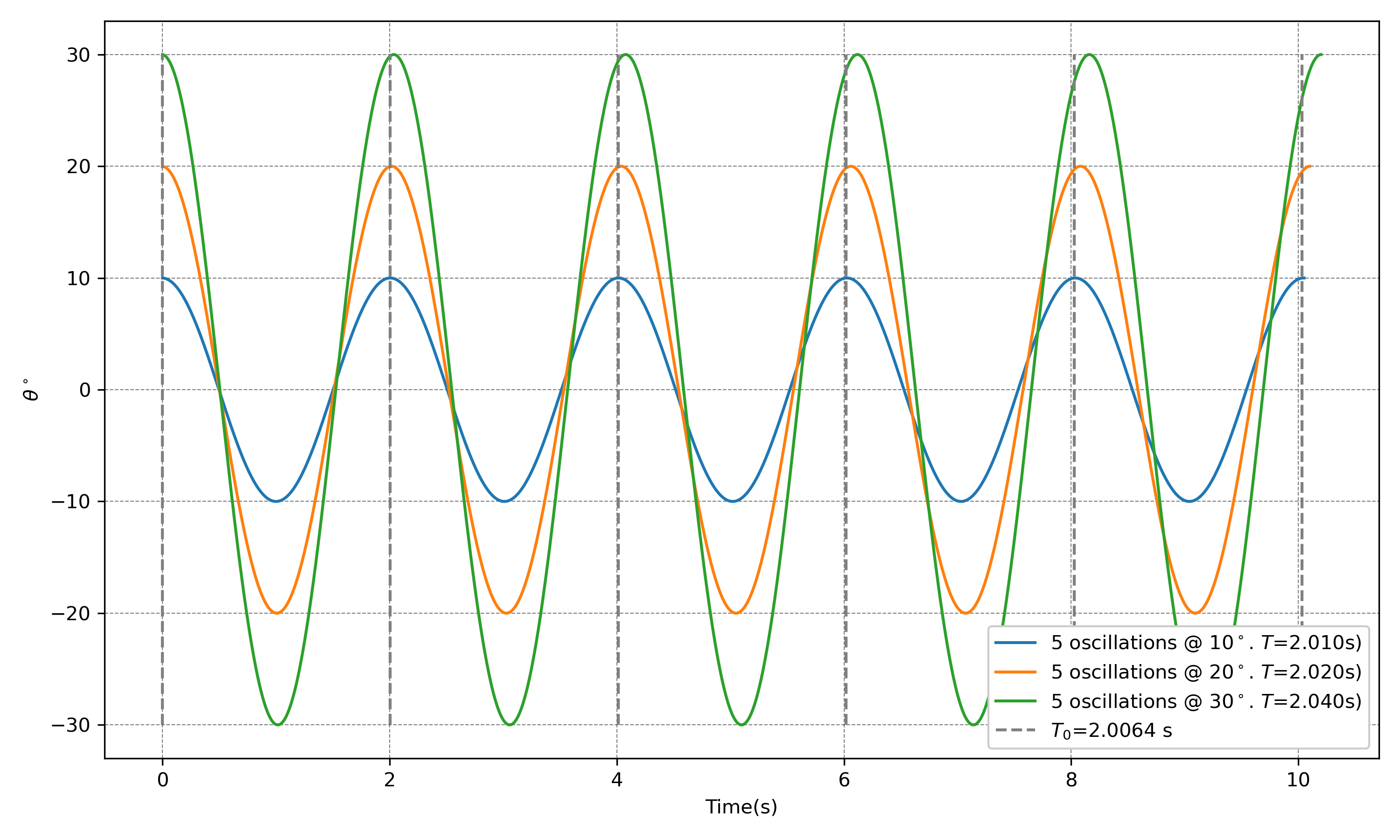
After the simulation, calculate the individual periods using
Here is what I obtained with my code.
Step 2: Add damping to the model
It is almost absurdly easy to incorporate damping: we only need to change the angular-acceleration term.
Our undamped model is
\[ \frac{d^2\theta}{dt^2} = -\frac{g}{L}\sin\theta. \]
I will model the damping as being proportional to the angular velocity. The damped model is
\[ \frac{d^2\theta}{dt^2} = -\frac{g}{L}\sin\theta -\gamma\frac{d\theta}{dt}, \tag{3}\]
where \(\gamma\) is the damping rate and has units of \(\mathrm{s^{-1}}\). Setting \(\gamma=0\) recovers our original undamped model.
Letting
\[ \omega=\frac{d\theta}{dt}, \]
we can write Equation 3 as two first-order equations:
\[ \begin{aligned} \frac{d\omega}{dt} &= -\frac{g}{L}\sin\theta-\gamma\omega,\\ \frac{d\theta}{dt} &= \omega. \end{aligned} \]{#eq-damped-pendulum-first-order
For velocity-first Euler–Cromer,
\[ \begin{aligned} \omega_{n+1} &= \omega_n+ \left[ -\frac{g}{L}\sin(\theta_n) -\gamma\omega_n \right]\Delta t,\\ \theta_{n+1} &= \theta_n+\omega_{n+1}\Delta t. \end{aligned} \tag{4}\]
In Python, the only change is:
The Euler–Cromer updates remain:
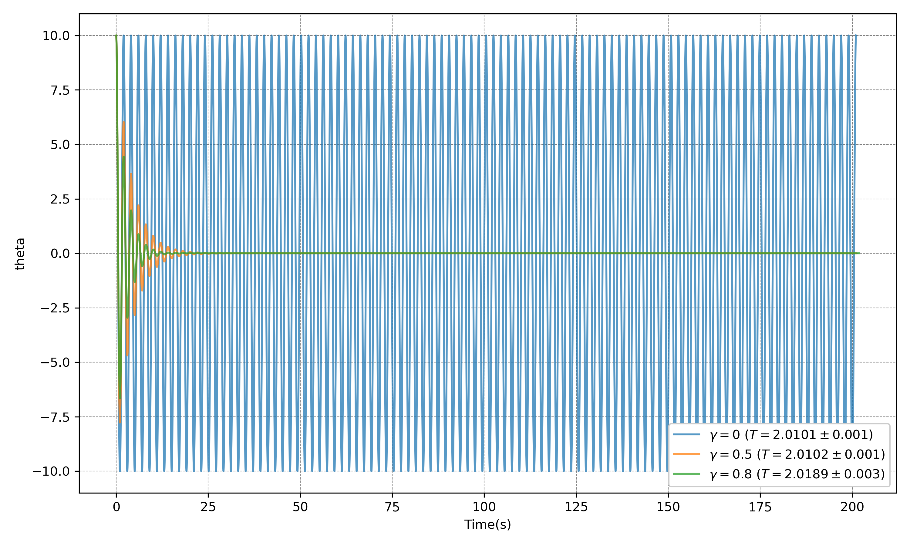
Start with \(\gamma=0.2\,\mathrm{s^{-1}}\) and compare the result with \(\gamma=0\). Here is what I obtained with my code for 20 oscillations.
3.2 Estimate \(\gamma\) for your experiment
Use trial and error to estimate \(\gamma\) from the amplitude decay in your \(10^\circ\) and \(20^\circ\) experiments.
For each starting angle:
- choose a value of \(\gamma\)
- run the simulation for the same number of oscillations as your experiment
- compare the simulated amplitude decay with your observations
- adjust \(\gamma\) until you obtain a reasonable match
There are more systematic approaches, such as bisection and optimisation, but I want to keep the complications to a minimum for now.
Ideally, one value of \(\gamma\) should describe both starting angles. If you obtain substantially different values, this may indicate that:
- the measurements are uncertain
- the damping is not proportional to angular velocity
- our model is missing another effect, such as dry friction
This is not a failure but useful information for our next modelling iteration. However, lets leave this for another time.
3.3 Period over successive oscillations
Use your estimated value of \(\gamma\) to simulate 30 oscillations starting from \(10^\circ\) and \(20^\circ\).
Plot the period of each oscillation against the oscillation number. Then ask:
- Does the period remain constant?
- Does it approach a limiting value as the amplitude decreases?
- Is the change large enough to matter experimentally?
- How do the results differ between starting angles of \(10^\circ\) and \(20^\circ\)?
4 Last task: How many oscillations should we have timed?
4.1 Timing uncertainty
In Week 1, we asked how many oscillations should be included in one timing measurement. We can now return to that question with a better understanding of the pendulum.
Timing more oscillations reduces the effect of reaction time. Suppose the uncertainty associated with each press of the stopwatch is \(\delta t\). Since we press it once to start and once to stop, the uncertainty in the total measured time is approximately
\[ \delta t_{\mathrm{total}} \approx \sqrt{2}\,\delta t. \tag{5}\]
If we time \(N\) oscillations, the uncertainty in the period is therefore
\[ \delta T \approx \frac{\sqrt{2}\,\delta t}{N}. \tag{6}\]
However, timing more oscillations also means that:
- the amplitude decreases
- the nonlinear period changes as the amplitude decreases
- out-of-plane motion and other imperfections may accumulate
- the motion eventually becomes difficult to observe
There is a trade-off: more oscillations reduce timing uncertainty, but give the pendulum more time to change.
Comparing two periods
We measured \(T_{10^\circ}\) and \(T_{20^\circ}\) independently. The approximate uncertainty in their difference is therefore
\[ \delta\left(T_{20^\circ}-T_{10^\circ}\right) = \sqrt{ \left(\delta T_{20^\circ}\right)^2 + \left(\delta T_{10^\circ}\right)^2 }. \]
If the two period measurements have similar uncertainties, then
\[ \delta\left(T_{20^\circ}-T_{10^\circ}\right) \approx \frac{2\delta t}{N}. \tag{7}\]
4.2 What you have to do:
Use \(\delta t=0.2\,\mathrm{s}\) in Equation 12 and stimate the uncertainty in one period measurement for \[ N=1,\ 5,\ 10,\ 20,\ \text{and}\ 30. \]
Use Equation 7 to estimate the uncertainty in \(T_{20^\circ}-T_{10^\circ}\).
Compare these uncertainties with the difference predicted by your model.
Use the damped model to determine how much the amplitude and period change over the same numbers of oscillations.
Recommend how many oscillations you would time if you repeated the Week 1 experiment.
Your recommendation should balance:
- timing precision
- amplitude decay
- the changing period
- the practical difficulty of observing the motion
#================================================================================================== ## Your task
- Add the damping term to your Euler–Cromer simulation.
- Begin with:
- \(L=1\,\mathrm{m}\)
- \(\theta(0)=20^\circ\)
- \(\omega(0)=0\)
- \(\gamma=0.2\,\mathrm{s^{-1}}\)
- \(\Delta t=0.01\,\mathrm{s}\)
- a total time of \(20\,\mathrm{s}\)
- Plot \(\theta(t)\) for both the damped and undamped models.
- Describe what changes and what remains approximately unchanged.
- Repeat using a few values of \(\gamma\), including \(0\), \(0.05\), \(0.2\), and \(0.5\,\mathrm{s^{-1}}\).
5 2. Extract the motion from a video
I have provided a common pendulum video and some starter Python code. You are welcome to use another tracking tool if you prefer:
- Tracker, designed specifically for video analysis in physics
- Fiji with TrackMate, a powerful general-purpose image and particle-tracking tool
- Kinovea, a video annotation and motion-analysis tool
- the Python tracking code that I have provided
I tried several approaches and eventually wrote my own Python code because that was simpler—for me. Please use whichever tool allows you to think most clearly about the science.
5.1 What you need from the video
For each frame, obtain:
- the time, \(t\)
- the horizontal position of the bob, \(x\)
- the vertical position of the bob, \(y\)
You will also need the position of the pivot, \((x_{\mathrm{p}},y_{\mathrm{p}})\).
If the image coordinate \(y\) increases downwards, calculate the angle using
\[ \theta(t) = \tan^{-1}\left( \frac{x(t)-x_{\mathrm{p}}} {y(t)-y_{\mathrm{p}}} \right). \]
In Python, use arctan2() rather than dividing the coordinates directly:
This gives the angle in radians. Convert it to degrees only when needed for presentation.
5.2 Check the tracking
Before doing anything sophisticated, plot \(\theta\) against time and ask:
- Does it oscillate around a sensible equilibrium position?
- Does the amplitude decrease?
- Are there sudden jumps or obviously incorrect points?
- Does the measured period look reasonable?
Do not rush past this step. A fitting algorithm will happily fit bad tracking data.
6 3. Estimate the damping rate
For weak damping, the amplitude decreases approximately as
\[ A(t)=A_0e^{-\gamma t/2}. \tag{9}\]
Taking logarithms,
\[ \ln A(t) = \ln A_0-\frac{\gamma}{2}t. \tag{10}\]
This turns the exponential decay into a straight-line problem. If the slope of a graph of \(\ln A\) against \(t\) is \(m\), then
\[ \gamma=-2m. \tag{11}\]
6.1 Your task
- Find the maxima of \(|\theta(t)|\).
- Plot these amplitudes against time.
- Plot \(\ln A\) against time.
- Fit a straight line and use Equation 11 to estimate \(\gamma\).
The appropriate value of prominence depends on your data. Plot the detected peaks and check them rather than trusting the function blindly.
6.2 Compare model and data
- Run your damped simulation using the value of \(\gamma\) obtained from the video.
- Use the measured initial angle and pendulum length.
- Plot the measured and simulated angles on the same axes.
- Compare:
- the period
- the decay of the amplitude
- the phase of the oscillations
- Identify where the model agrees with the data and where it fails.
7 4. How many oscillations should we have timed?
In Week 1, we asked how many oscillations should be included in a timing measurement. We can now return to that question with a better understanding of the pendulum.
Timing more oscillations reduces the effect of reaction time on the period. If the uncertainty in starting and stopping the timer is approximately \(\delta t\), then the uncertainty in the period obtained from \(N\) oscillations is roughly
\[ \delta T \approx \frac{\sqrt{2}\,\delta t}{N}. \tag{12}\]
However, timing more oscillations also means that:
- the amplitude decreases
- the nonlinear period changes slightly as the amplitude changes
- out-of-plane motion and other imperfections may accumulate
- the signal eventually becomes difficult to observe
There is therefore a trade-off: more oscillations reduce random timing uncertainty, but may increase the influence of model and procedural changes.
7.1 Your final task
- Use \(\delta t=0.2\,\mathrm{s}\) in Equation 12.
- Estimate the timing uncertainty for \(N=1\), \(5\), \(10\), \(20\), and \(30\) oscillations.
- Compare these values with your predicted difference \(T_{20^\circ}-T_{10^\circ}\).
- Use the damped model to examine how much the amplitude changes over the same number of oscillations.
- Recommend how many oscillations you would time if you repeated the Week 1 experiment.
Your recommendation must balance:
- timing precision
- amplitude decay
- the changing period
- the practical difficulty of the measurement
There may not be one perfect answer. What matters is that your recommendation is supported by evidence.
8 What to report
By the end of the session, your group should have:
- a plot comparing damped and undamped simulations
- an estimate of \(\gamma\) from the common video
- a plot comparing the damped model with the video data
- a brief answer to whether damping changes the period appreciably
- a justified recommendation for how many oscillations should be timed
Footnotes
Or not.↩︎