force = 10.0       # N
mass = 2.0         # kg
dt = 0.01          # s

acceleration = force / mass

time = 0.0
initial_position = 0.0
initial_velocity = 0.0

position = initial_position
velocity = initial_velocity

# =========== Simulate using  Euler =========== #
history = [[time, position, velocity]]

while position < 1000:  # Stop after travelling 1 km
    position += velocity * dt
    velocity += acceleration * dt
    time += dt

    history.append([time, position, velocity])
# ============================================ #

# Extract the simulation results
t, x, v = np.array(history).T

# Calculate the analytical result at the same times
x_analytical = (
    initial_position
    + initial_velocity * t
    + 0.5 * acceleration * t**2
)

# Compare the results
plt.plot(t, x, label="Displacement (Euler)")
plt.plot(t, x_analytical, linestyle="--", label="Displacement (analytical)")

plt.xlabel("Time (s)")
plt.ylabel("Displacement (m)")
plt.legend()
plt.show()Numerically modelling the simple pendulum I
Activity 1 | Week 3 | Lecture
\[ % \newcommand\v[1]{\vec{#1}} % \newcommand\v[1]{\mathbf{#1}} \newcommand\v[1]{\boldsymbol{#1}} \newcommand\vdot[2]{\v{#1}\cdot\v{#2}} \]
\[ \newcommand{\dd}[2][]{\mathrm{d}^{#1}#2} \]
\[ \newcommand\f[2]{\dfrac{#1}{#2}} \newcommand\da[2]{\dfrac{d #1}{d #2}} \newcommand\daa[2]{\dfrac{d^2 #1}{d #2^2}} \newcommand\pa[2]{\dfrac{\partial #1}{\partial #2}} \newcommand\paa[2]{\dfrac{\partial^2 #1}{\partial #2^2}} \newcommand\pab[3]{\dfrac{\partial^2 #1}{\partial #2 \partial #3}} \def\half{\frac{1}{2}} \]
\[ \newcommand\ket[1]{\left|#1\right\rangle} % |x> \newcommand\exp[1]{\left\langle#1\right\rangle} % <x> \newcommand\lr[1]{\left(#1\right)} % (x) \newcommand\lrs[1]{\left[#1\right]} % [x] %\newcommand\lrb[1]{\left|#1\right|} % |x| \newcommand\lra[1]{\left|#1\right|} % |x| \newcommand\lrc[1]{\left\{#1\right\}} % {x} \newcommand\lrl[3]{\left.#1\right|_{#2}^{#3}} % x_limits \]
\[ \def\ie{\text{i.e.}\quad} \]
$$ % Typical reaction % Nuclear reactions
$$
\[ \newcommand{\coulomb}[1]{\dfrac{#1}{4\pi\epsilon_0}} \]
\[ \def\amu{\text{ amu}} \def\J{\text{ J}} \def\K{\text{ K}} \def\s{\text{ s}} \def\second{\text{ s}} \def\Psecond{\text{ s}^{-1}} \def\m{\text{ m}} \def\mm{\text{ mm}} \def\km{\text{ km}} \def\fm{\text{ fm}} \def\mum{\text{ $\mu$m}} \def\mus{\text{ $\mu$s}} \def\mPERs{\text{ ms$^{-1}$}} \def\eV{\text{ eV}} \def\keV{\text{ keV}} \def\GeV{\text{ GeV}} \def\MeV{\text{ MeV}} \def\MeVc{\text{ MeV/c$^2$}} \def\KeVc{\text{ KeV/c$^2$}} \newcommand\ttp[1]{\times 10^{#1}} % To The Power \]
$$
$$
\[ \def\uraniumA{_{92}^{233}{\text{U}}_{}} \def\uraniumB{_{92}^{235}{\text{U}}_{}} \def\uraniumC{_{92}^{238}{\text{U}}_{}} \def\carbonB{_{6}^{14}{\text{C}}_{}} \def\nitrogenB{_{7}^{14}{\text{N}}_{}} \def\oxygenA{_{8}^{14}{\text{O}}_{}} \def\oxygenB{_{8}^{16}{\text{O}}_{}} \]
\[ \def\com{\text{\scriptsize CM}} \]
\[ \def\l{\ell} \def\l{l} \]
\[ \def\g{\gamma} \def\g{\gamma} \]
1 What to expect
1.1 Story so far
Over the past two weeks, we have spent a great deal of time measuring and modelling the period of a pendulum. Our measurements provided evidence that the periods at \(10^\circ\) and \(20^\circ\) are different.
To strengthen this experimental result, we developed the mathematical model
\[ \frac{d^2\theta}{dt^2} = -\frac{g}{L}\sin\theta. \tag{1}\]
We then explored the small-angle approximation, which predicts
\[ T=2\pi\sqrt{\frac{L}{g}}. \tag{2}\]
This is a wonderfully simple result, but the amplitude does not appear in it. The approximation therefore predicts that \(T_{10^\circ}\) and \(T_{20^\circ}\) are identical. Yet our measurements provide some evidence to the contrary.
So, we must return to Equation 1. Solving it analytically requires mathematics that is beyond what we need here. Instead, I will show you how to construct a very accessible numerical solution that can support and complement our measurements.
1.2 Euler to the rescue
Euler’s method, which you first encountered in 73 and will use again for Daisyworld in 75, begins with a simple idea. Over a small interval \(\Delta x\), we can write
\[ \frac{dy}{dx} \approx \frac{\Delta y}{\Delta x}. \]
Rearranging,
In words: if we know the present value of \(y\) and its rate of change, we can estimate what \(y\) will be after a small step.
For the pendulum, let
\[ \omega=\frac{d\theta}{dt} \]
be the instantaneous angular velocity. We can then rewrite Equation 1 as
\[ \begin{aligned} \frac{d\omega}{dt} &= -\frac{g}{L}\sin\theta,\\ \frac{d\theta}{dt} &= \omega. \end{aligned} \]
Over a small time step \(\Delta t\),
\[ \begin{aligned} \Delta\omega &\approx -\frac{g}{L}\sin\theta\,\Delta t,\\ \Delta\theta &\approx \omega\,\Delta t. \end{aligned} \tag{4}\]
These two expressions give us a numerical strategy: update the angular velocity, update the angle, and repeat.
2 Warming up
Before tackling the pendulum, let’s warm up by first using Euler’s method on a simpler problem.
Imagine a box of mass \(m\) pushed by a constant force \(F\). The box has a constant acceleration, so its speed continually increases. As it speeds up, it also travels further during each time step.
Newton’s second law gives
\[ F = ma = m\frac{dv}{dt} = m\frac{d^2x}{dt^2}. \]
2.1 Solving analytically
I chose this toy problem because we can easily solve it analytically.
Since
\[ a=\frac{F}{m}, \tag{5}\]
and the box begins at position \(x_0\) with velocity \(u\), the solution is
\[ \begin{aligned} v(t)&=u+at,\\[1em] x(t)&=x_0+ut+\frac{1}{2}at^2. \end{aligned} \tag{6}\]
Velocity
Beginning with the acceleration,
\[ \frac{dv}{dt}=a. \]
Integrating from the initial velocity \(u\) at \(t=0\) to the velocity \(v(t)\) at time \(t\),
\[ \begin{aligned} \int_u^{v(t)}dv' &= \int_0^t a\,d{t},\\ v(t)-u &= at. \end{aligned} \]
Therefore,
\[ v(t)=u+at. \]
Displacement
Since \(v=dx/dt\),
\[ \frac{dx}{dt}=u+at. \]
Integrating again,
\[ \begin{aligned} \int_{x_0}^{x(t)}dx &= \int_0^t (u+at)\,dt,\\ x(t)-x_0 &= ut+\frac{1}{2}at^2. \end{aligned} \]
Therefore,
\[ x(t)=x_0+ut+\frac{1}{2}at^2. \]
2.2 Solving using Euler
To use Euler’s method:
Step 1: Re-write the motion as two first-order equations:
\[ \begin{align} a&=\frac{dv}{dt}=\frac{F}{m}\\[2em] v&=\frac{dx}{dt}. \end{align} \tag{7}\]
Step 2: Over a small time step \(\Delta t\) approximate,
\[ \begin{align} \Delta v & \approx\frac{F}{m}\Delta t,\\[2em] \Delta x & \approx v\Delta t. \end{align} \tag{8}\]
Implementing in Python
Let’s implement Euler in Python for our toy problem. Please note how we use the state now (speed and acceleration) to estimate the next state.
Here is the typical code.
If you run this with different, values for time-steps (dt) you will get the following results shown in Figure 1. Notice how the accuracy of the result depends on the value of dt.
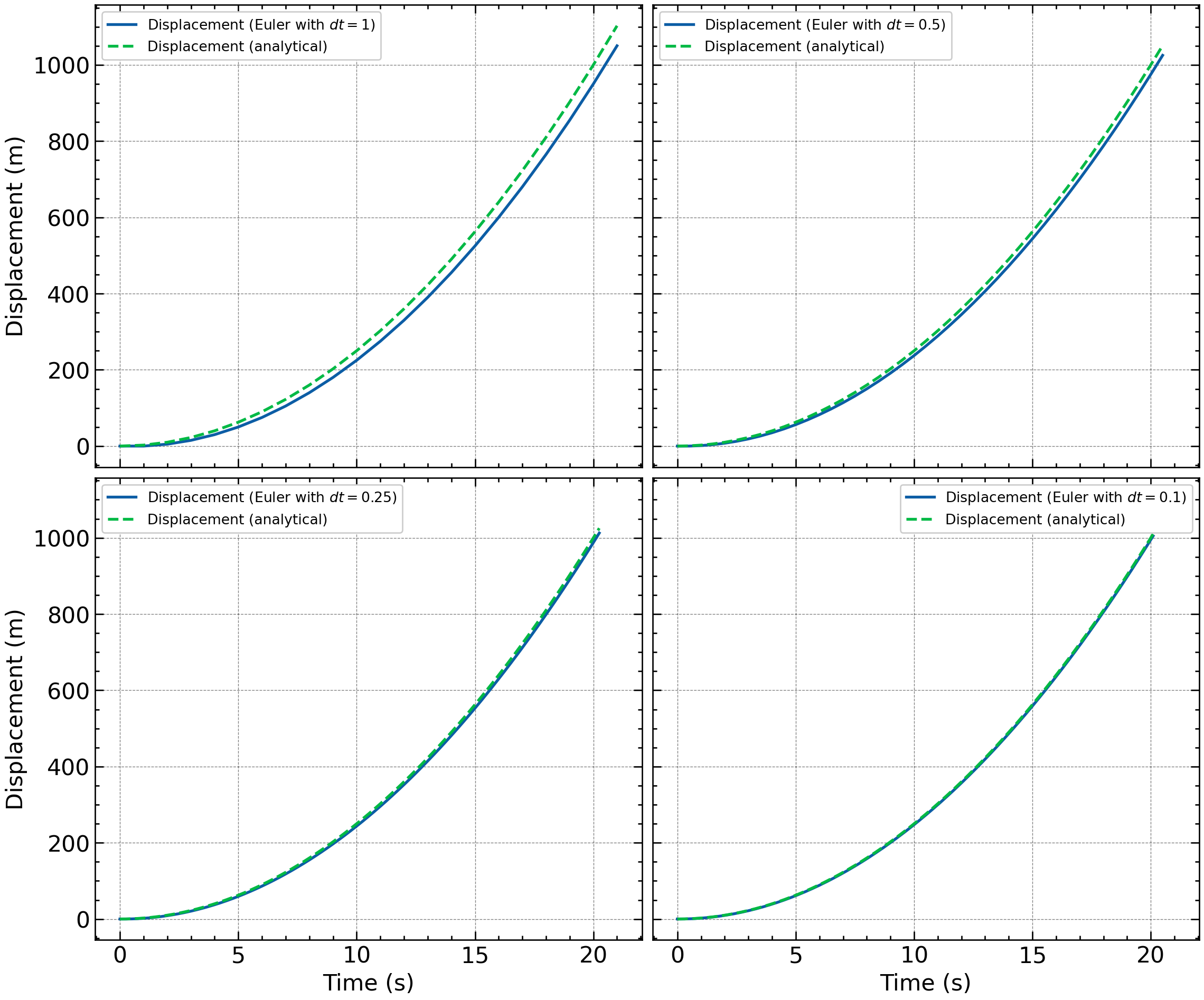
dt
2.3 Beyond Euler
I am introducing Euler’s method first because it allows us ‘get a feel’ for the system we are studying by building a simulation one step at a time. Once the model makes sense and we want greater accuracy and efficiency, we need alternatives.
Standard Python packages such as SciPy provide highly optimised, higher-order numerical solvers that you can unleash on your problems. You encountered one of these, odeint(), in 73. Let me now introduce you to its more modern cousin: solve_ivp().
Let me demonstrate it using our toy box problem.
solve_ivp() expects us to provide:
- the differential equations
- the initial conditions
- the time interval over which we want a solution
We express these equations as a Python function.
First, lets load the solver.
The differential equations
The first returned value is \(dx/dt\), while the second is \(dv/dt\).
Time interval of the simulation
I would like the simulation to stop when the box reaches \(1\,\mathrm{km}\). We can define this as an event reach_one_kilometre() which must return a zero at the event.
Initial conditions
Now we can solve the equations:
Unlike our Euler code, solve_ivp() chooses its time steps adaptively. I.e. it takes smaller steps when the solution needs more care and larger steps when the solution is changing smoothly. Here, max_step limits the largest step it may take; it does not force every step to have that size.
Since we know the analytical solution, we can check the results. This is shown in Figure 2
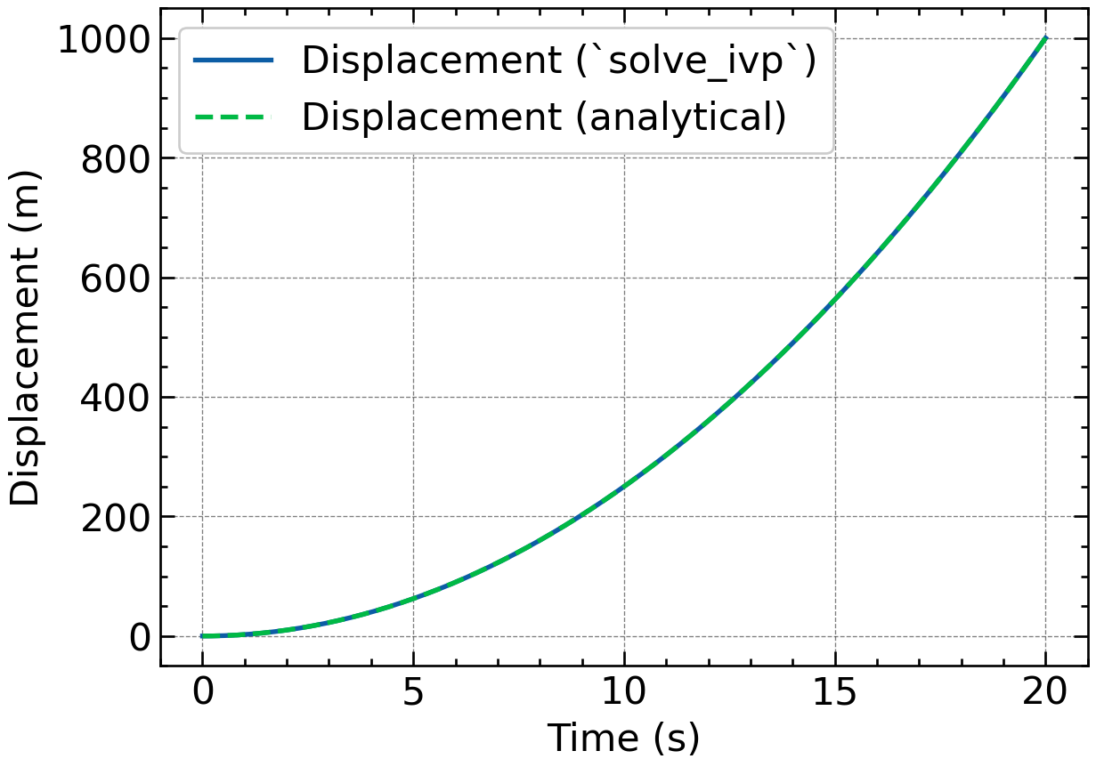
solve_ivp() and the analytical solution.
When we want energy conservation, there is a family of methods called symplectic integrators. These methods do not conserve energy exactly, but they usually keep the energy error bounded (i.e. varying about a mean) rather than allowing it to drift continuously.
Let me show you one of the simplest: symplectic Euler, also called the Euler–Cromer method.
2.4 A symplectic Euler model
Euler–Cromer makes one tiny but crucial change to forward Euler:
- calculate the new velocity using the old position
- calculate the new position using the new velocity
That’s it!
Notice the order: I update the velocity first and then use that new velocity to update the position. This small change generally produces much more sensible long-term behaviour for an oscillating system.
3 Finding the period
Unlike an analytical function, a numerical solution contains only a finite set of points. It is unlikely that a peak or zero crossing will always fall exactly one of the points in this finite set of numbers. So, before we dig into the pendulum simulation, I want to show you two strategies for finding the period of a numerical solution.
- writing our own zero-crossing function
- using
find_peaks()from SciPy
To see how they work, let us use a simple sine curve, whose period we know is \(T=2\pi = 360^\circ\).
3.1 Using zero crossings
One way to determine the period is to find successive events where the signal crosses zero in the same direction.
The following function finds positive-to-negative crossings by interpolation between the two points as seen in Figure 3. \[ \f{y_1}{x_0-x_1} = \f{-y_2}{x_2-x_0} \Rightarrow x_0 = \f{y_1x_2-y_2x_1}{y_1-y_2} \tag{9}\]
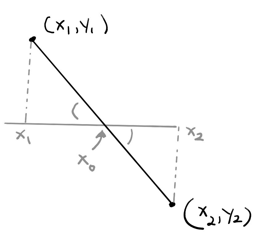
We can now estimate the period:
crossings = downward_zero_crossings(x, y)
periods = np.diff(crossings)

period_mean = periods.mean()
period_std = periods.std(ddof=1)

print(f"Expected period: {np.rad2deg(2 * np.pi):.6f}")
print(f"Mean period: {np.rad2deg(period_mean): .6f}")
print(f"Standard deviation: {np.rad2deg(period_std):.2e}")
Expected period: 360.000000
Mean period: 360.000000
Standard deviation: 3.17e-063.2 Using find_peaks()
SciPy’s find_peaks() function is more convenient approach because it identifies the local maxima of the signal:
from scipy.signal import find_peaks

peaks, properties = find_peaks(y)

peak_positions = x[peaks]
periods = np.diff(peak_positions)

period_mean = periods.mean()
period_std = periods.std(ddof=1)

print(f"Expected period: {np.rad2deg(2 * np.pi):.6f}")
print(f"Mean period: {np.rad2deg(period_mean): .6f}")
print(f"Standard deviation: {np.rad2deg(period_std):.2e}")
Expected period: 360.000000
Mean period: 359.965883
Standard deviation: 2.96e-01We can check what find_peaks() detected by adding the peaks to the plot:
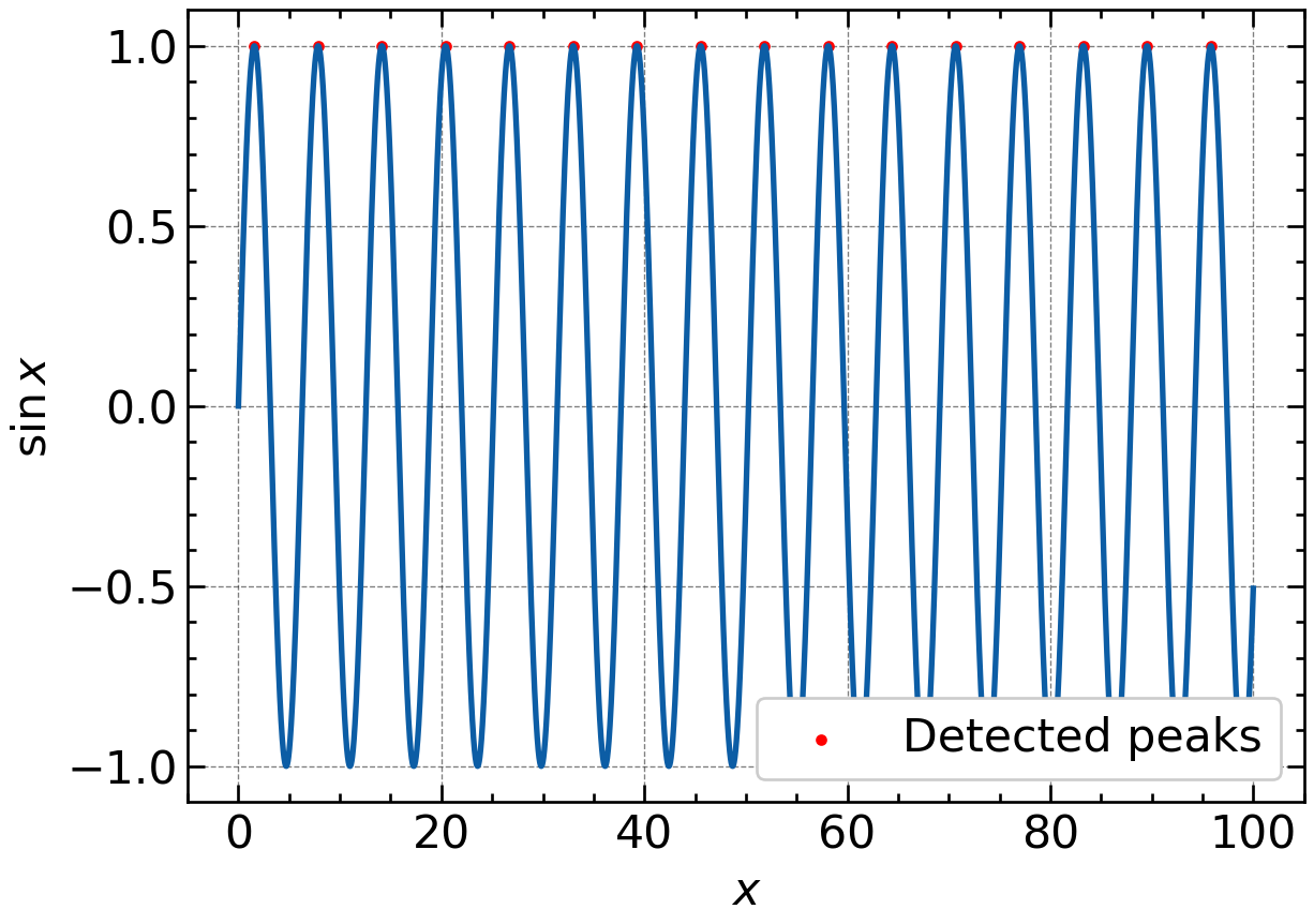
find_peaks()
Note:
- For the pendulum, replace
xwith the simulation time andywith the simulated angle. - Whichever method you use, estimate the period across several cycles by running the simulation for longer.
- Although
find_peaks()performs less well for this particular dataset, it offers useful options for dealing with noisy data. So, do not rush to discard it.
4 Simulating the pendulum; your turn!
It is now your turn to simulate the pendulum. We will proceed in stages so that you can see what works, what fails, and how to improve it.
4.1 Build the simulation
Implement Equation 4 using forward Euler.
Use:- \(L=1\) m
- \(g\) from
scipy.constants(from scipy.constants import g) - \(\theta(0)=10^\circ\)
- \(\omega(0)=0\)
- a simulation time of at least \(10\,\mathrm{s}\)
Remember to convert the starting angle to radians before using
np.sin().Plot \(\theta\) against time. What happens to the amplitude? Is this physically sensible?
Fix the obvious problem by replacing forward Euler with the Euler–Cromer method. Plot the result again and compare the two simulations.
Determine the period from your Euler–Cromer simulation. Measure across several oscillations rather than relying on only one.
Repeat the simulation using progressively smaller values of \(\Delta t\). Continue until the period is stable to a precision that you consider adequate.
4.2 Investigate the small-angle approximation
Use your converged Euler–Cromer simulation to answer the following:
Determine the period for a starting angle of \(10^\circ\).
Compare it with the small-angle prediction
\[ T_0=2\pi\sqrt{\frac{L}{g}}. \tag{10}\]
Temporarily replace
np.sin(angle)\(\longrightarrow\)angleand determine the period again.Compare the three results:
- the nonlinear simulation using \(\sin\theta\)
- the numerical small-angle simulation using \(\theta\)
- the analytical small-angle prediction, \(T_0\)
How far off is the small-angle approximation? Report both the absolute and percentage differences.
4.3 Compare \(T_{10^\circ}\) and \(T_{20^\circ}\)
Reset the code to the original nonlinear model containing \(\sin\theta\).
Determine \(T_{10^\circ}\) and \(T_{20^\circ}\) using the same converged value of \(\Delta t\).
Calculate \[ T_{20^\circ}-T_{10^\circ}. \]
Express this difference as a percentage of \(T_{10^\circ}\).
Compare your numerical results with the first analytical correction:
\[ T(\theta_0) \approx T_0\left(1+\frac{\theta_0^2}{16}\right), \tag{11}\]
Remember \(\theta_0\) must be expressed in radians.
Finally, compare the predicted difference with the uncertainty in your experimental measurements. Was your experiment precise enough to detect it?
4.4 Finding the period
The positive peaks correspond to the pendulum returning to the same maximum angle. The time between successive peaks is therefore one period.
Let us now compare several starting angles:
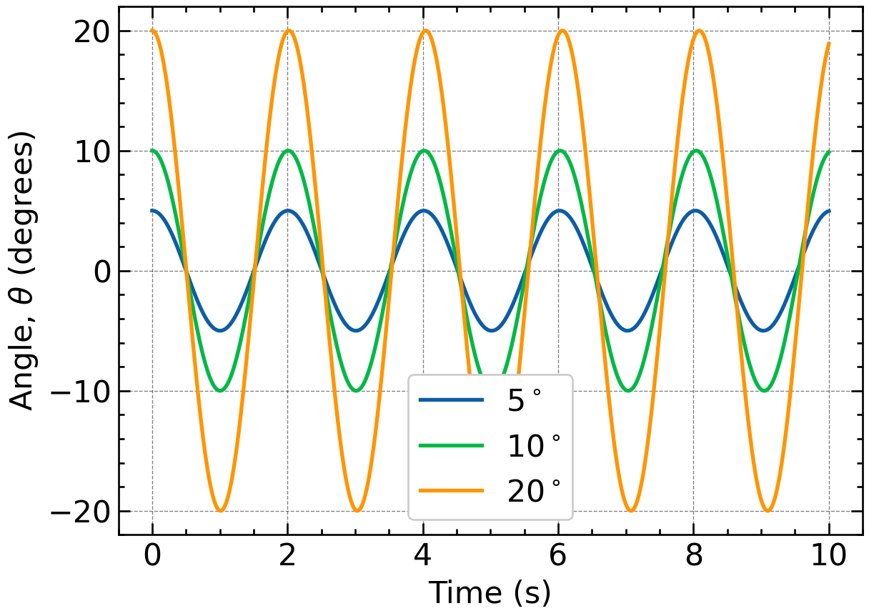
A typical result for a \(1\,\mathrm{m}\) pendulum is:
| Starting angle | Predicted period |
|---|---|
| \(5^\circ\) | \(2.0074\,\mathrm{s}\) |
| \(10^\circ\) | \(2.0102\,\mathrm{s}\) |
| \(20^\circ\) | \(2.0218\,\mathrm{s}\) |
Therefore,
\[ T_{20^\circ}-T_{10^\circ} \approx 0.0116\,\mathrm{s}. \]
This is a relative difference of only
\[ \frac{T_{20^\circ}-T_{10^\circ}} {T_{10^\circ}} \times100\% \approx0.58\%. \]
That is not a large difference. Your experimental challenge is to determine whether your measurements are precise enough to detect it.
4.5 Where we have arrived
We began with an experimental question and added a physical model. The small-angle approximation gave us a simple analytical result, but it could not explain the difference between \(T_{10^\circ}\) and \(T_{20^\circ}\). Returning to the full equation and solving it numerically gave us a testable prediction:
\[ T_{20^\circ}-T_{10^\circ}\approx0.012\,\mathrm{s}. \]
We can now return to the experiment with a much clearer target. We are no longer working blind.