Modelling the simple pendulum
Activity 1 | Week 2 | Lecture
\[ % \newcommand\v[1]{\vec{#1}} % \newcommand\v[1]{\mathbf{#1}} \newcommand\v[1]{\boldsymbol{#1}} \newcommand\vdot[2]{\v{#1}\cdot\v{#2}} \]
\[ \newcommand{\dd}[2][]{\mathrm{d}^{#1}#2} \]
\[ \newcommand\f[2]{\dfrac{#1}{#2}} \newcommand\da[2]{\dfrac{d #1}{d #2}} \newcommand\daa[2]{\dfrac{d^2 #1}{d #2^2}} \newcommand\pa[2]{\dfrac{\partial #1}{\partial #2}} \newcommand\paa[2]{\dfrac{\partial^2 #1}{\partial #2^2}} \newcommand\pab[3]{\dfrac{\partial^2 #1}{\partial #2 \partial #3}} \def\half{\frac{1}{2}} \]
\[ \newcommand\ket[1]{\left|#1\right\rangle} % |x> \newcommand\exp[1]{\left\langle#1\right\rangle} % <x> \newcommand\lr[1]{\left(#1\right)} % (x) \newcommand\lrs[1]{\left[#1\right]} % [x] %\newcommand\lrb[1]{\left|#1\right|} % |x| \newcommand\lra[1]{\left|#1\right|} % |x| \newcommand\lrc[1]{\left\{#1\right\}} % {x} \newcommand\lrl[3]{\left.#1\right|_{#2}^{#3}} % x_limits \]
\[ \def\ie{\text{i.e.}\quad} \]
$$ % Typical reaction % Nuclear reactions
$$
\[ \newcommand{\coulomb}[1]{\dfrac{#1}{4\pi\epsilon_0}} \]
\[ \def\amu{\text{ amu}} \def\J{\text{ J}} \def\K{\text{ K}} \def\s{\text{ s}} \def\second{\text{ s}} \def\Psecond{\text{ s}^{-1}} \def\m{\text{ m}} \def\mm{\text{ mm}} \def\km{\text{ km}} \def\fm{\text{ fm}} \def\mum{\text{ $\mu$m}} \def\mus{\text{ $\mu$s}} \def\mPERs{\text{ ms$^{-1}$}} \def\eV{\text{ eV}} \def\keV{\text{ keV}} \def\GeV{\text{ GeV}} \def\MeV{\text{ MeV}} \def\MeVc{\text{ MeV/c$^2$}} \def\KeVc{\text{ KeV/c$^2$}} \newcommand\ttp[1]{\times 10^{#1}} % To The Power \]
$$
$$
\[ \def\uraniumA{_{92}^{233}{\text{U}}_{}} \def\uraniumB{_{92}^{235}{\text{U}}_{}} \def\uraniumC{_{92}^{238}{\text{U}}_{}} \def\carbonB{_{6}^{14}{\text{C}}_{}} \def\nitrogenB{_{7}^{14}{\text{N}}_{}} \def\oxygenA{_{8}^{14}{\text{O}}_{}} \def\oxygenB{_{8}^{16}{\text{O}}_{}} \]
\[ \def\com{\text{\scriptsize CM}} \]
\[ \def\l{\ell} \def\l{l} \]
\[ \def\g{\gamma} \def\g{\gamma} \]
“All models are wrong, but some are useful”
– George Box
What to expect
In Week 1, you measured \(T_{10^\circ}\) and \(T_{20^\circ}\) and asked whether they were distinguishable within experimental uncertainty.
However, we were working somewhat “blind”: we had no theoretical prediction against which to assess our measurements.
In this lecture, I will show you how to construct a physical model of the pendulum and use it to better understand our experiment.
1 Constructing the physical model
1.1 Assumptions
Allow me to be explicit about the assumptions behind our simple-pendulum model:
- The bob is a point mass \(m\). We treat all its mass as concentrated at its centre. This is reasonable when the bob is small compared with the pendulum length.
- The string is light and does not stretch.
- Its length \(L\) remains constant under the tensions involved.
- Its mass is negligible compared with the mass of the bob.
- The pivot is fixed. If the pivot moves, we no longer have a simple pendulum.
- Air resistance and friction are negligible. This is a useful place to start, although we may need to reconsider it later.
- The pendulum moves in one vertical plane. We must try to ensure this experimentally.
- Gravity is uniform. This is reasonable because the pendulum is tiny compared with the Earth.
The pendulum ar rest
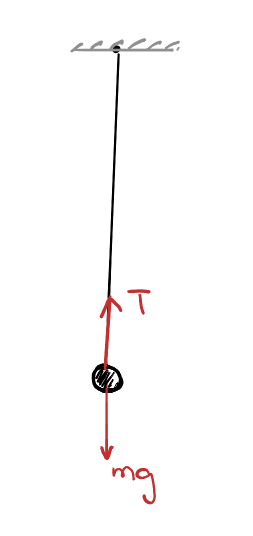
Let me begin with the simplest case: a pendulum at rest.
Two forces act on the bob:
- the tension, \(T\), acting upwards along the string
- its weight, \(mg\), acting downwards
The bob is in equilibrium. I like to think of this as the pendulum’s happy place: in our ideal model, it will remain there indefinitely unless disturbed.
Taking upwards as positive and applying Newton’s second law,
\[ \begin{aligned} F_{\mathrm{net}} &= ma,\\ T-mg &= 0,\\ \Rightarrow T=mg. \end{aligned} \]
This result applies while the pendulum is at rest. Once it begins to swing, the tension need not equal its weight.
The pendulum in motion
Now let us consider the more interesting case. If I disturb the pendulum from its happy place and release it, gravity pulls it back towards equilibrium. Gravity therefore provides a restoring force.
The pendulum does not stop when it first reaches equilibrium. By then it has kinetic energy and is moving at its greatest speed, so it carries on past its happy place. Gravity then pulls it back again, producing an oscillation.
This kind of motion is extremely common. Oscillations are also the building blocks from which we will develop our understanding of waves.
To analyse the motion, it helps to resolve the forces into two perpendicular directions as showm in Figure 2:
- the radial direction, along the string
- the tangential direction, along the bob’s path
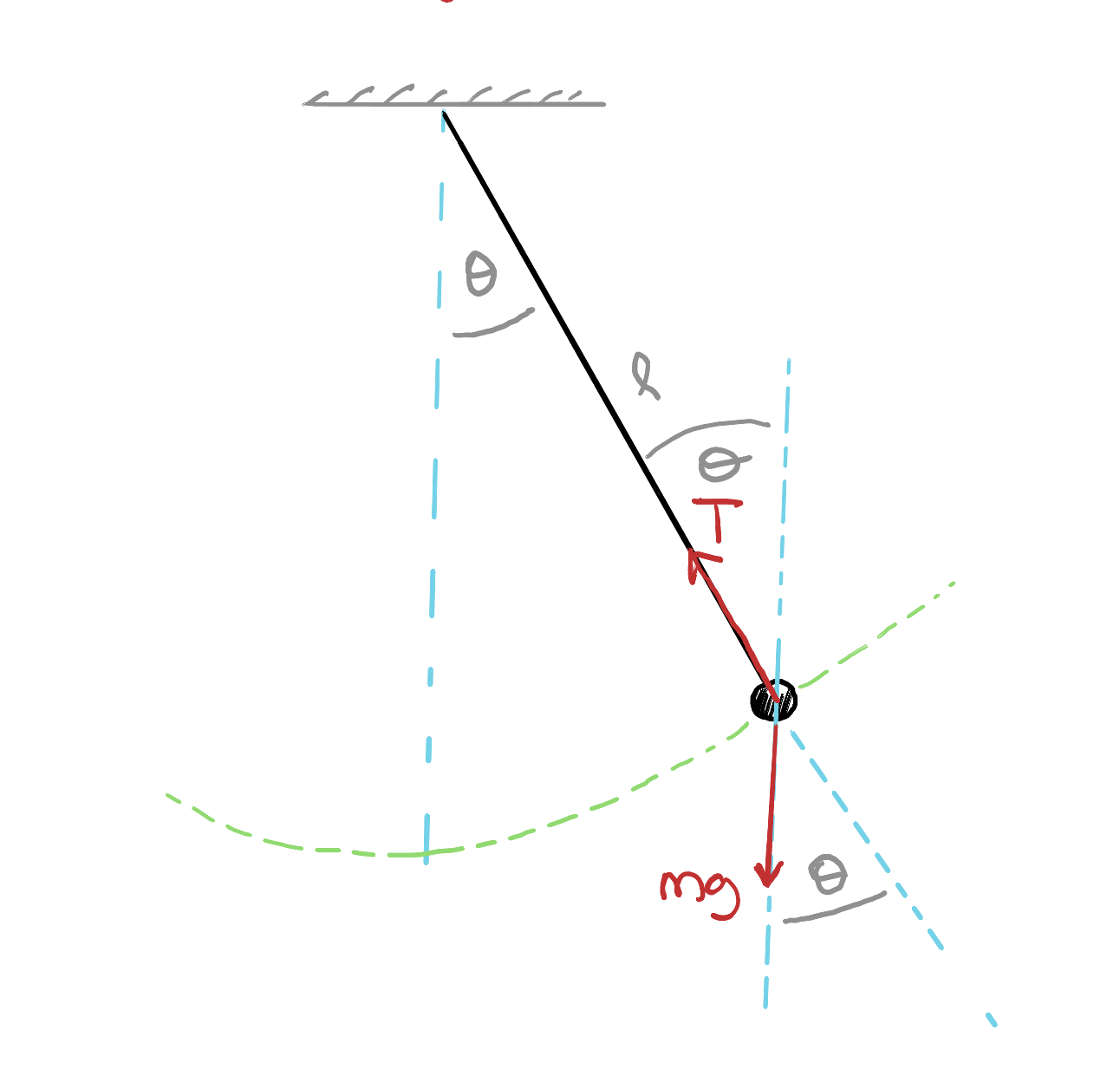
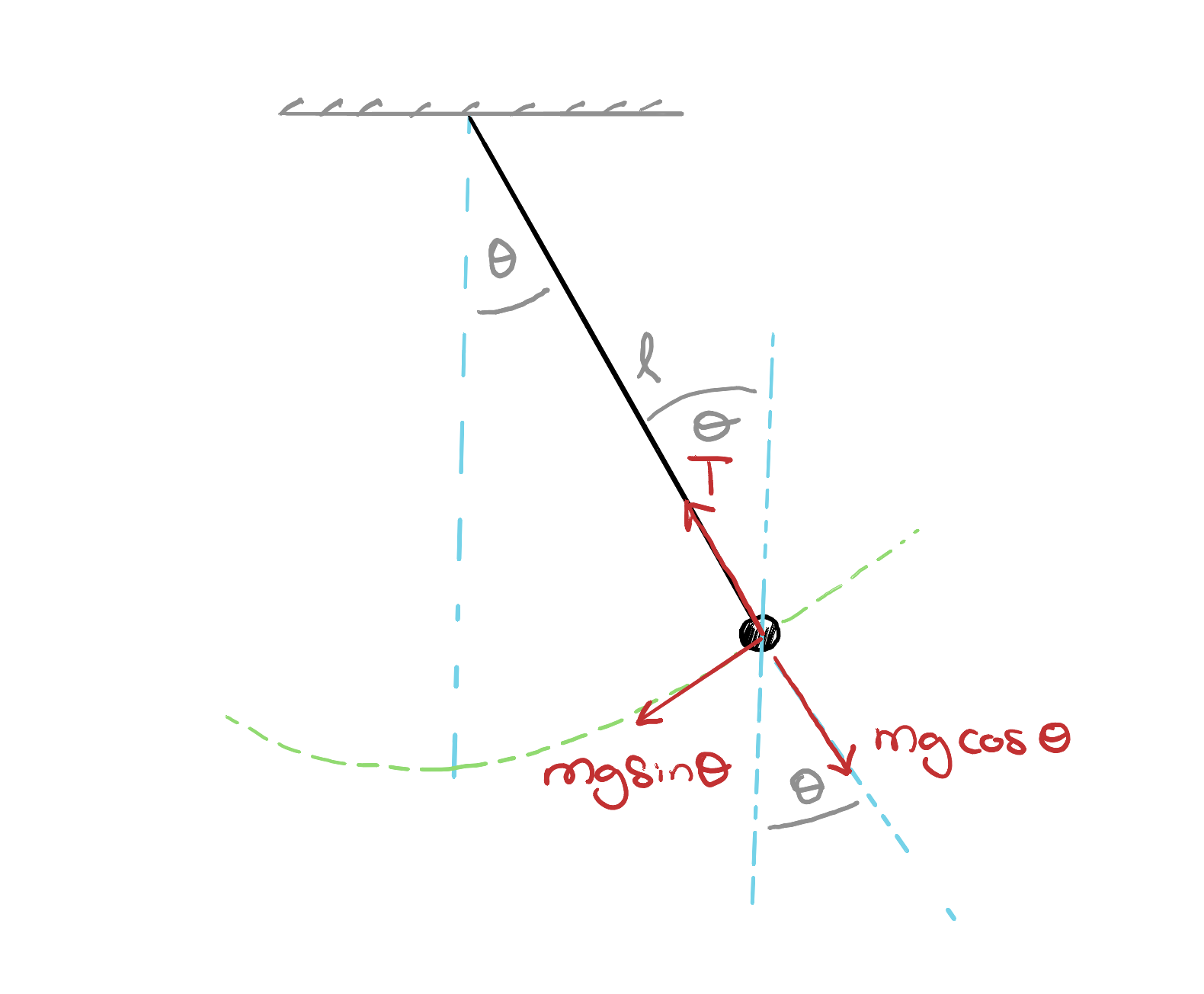
The tension acts radially, so it does not contribute to the tangential motion. The tangential component of the bob’s weight is
\[ F_{\mathrm{t}}=-mg\sin\theta. \tag{1}\]
Notice two things:
- the force always points towards the happy place
- its magnitude increases with the size of the angle, over the range \(-90^\circ \leq \theta \leq 90^\circ\) which is the range relevant to our pendulum.
The negative sign in Equation 1 tells us that the force acts opposite to the displacement \(\theta\).
The angular acceleration is \(\dfrac{d^2\theta}{dt^2}\). Because the bob moves along a circular path of radius \(L\), there is a corresponding tangential acceleration \[ a_{\mathrm{t}} = L\frac{d^2\theta}{dt^2}. \tag{2}\]
Applying Newton’s second law in the tangential direction,
\[ mL\frac{d^2\theta}{dt^2} = -mg\sin\theta. \]
The mass cancels, giving the differential equation that represents our model of the pendulum:
1.2 Can we solve it?
Equation 11 is a nonlinear differential equation. An exact expression for the period exists, but it involves an elliptic integral. Rather than introducing that machinery now, let us first try an approximate solution.
1.3 The small-angle approximation
For small angles, measured in radians, we can truncate the Taylor expansion of \(\sin \theta\), to get
\[ \sin\theta\approx\theta. \tag{4}\]
How good is the approximation?
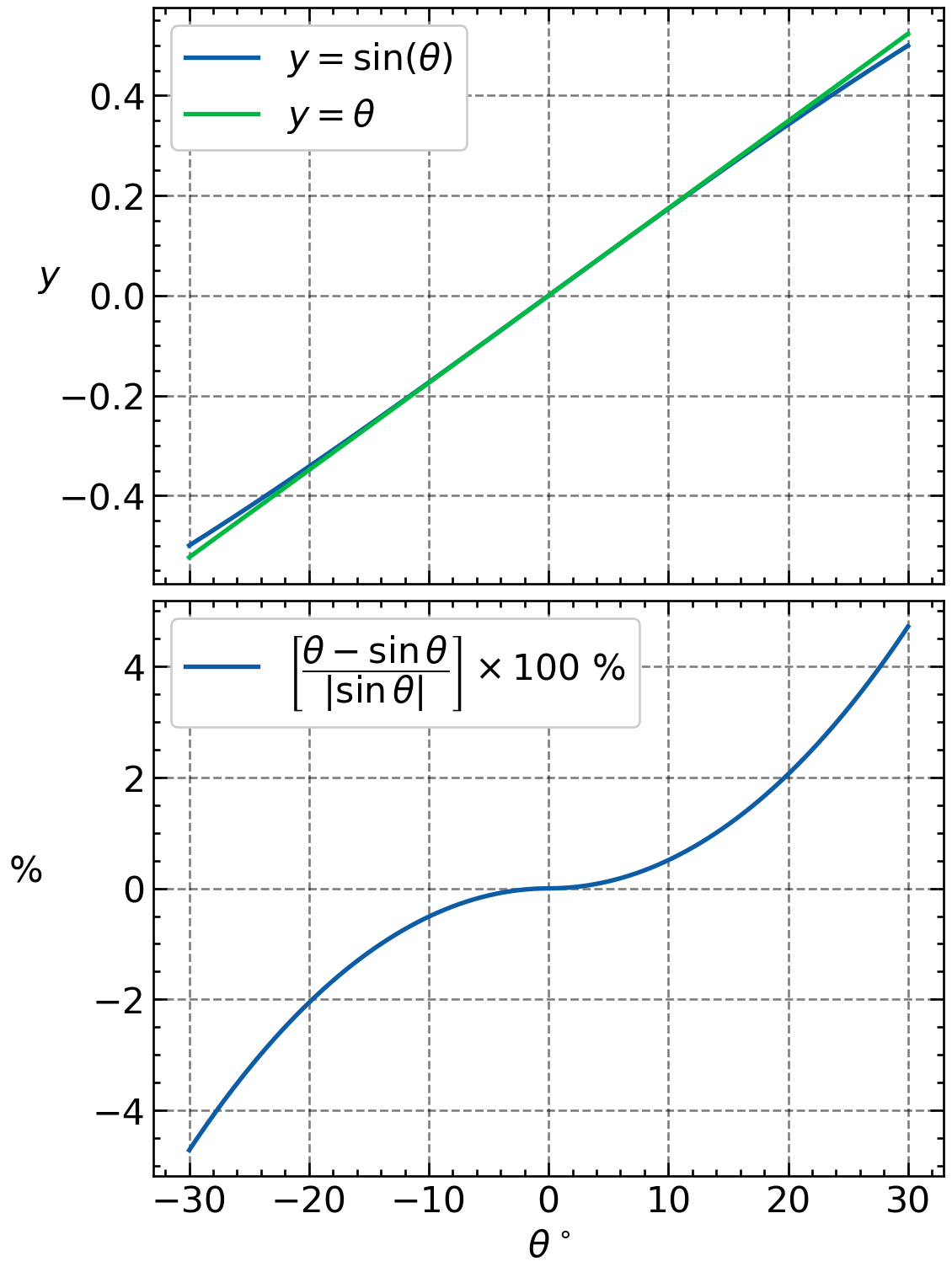
How ‘small’ is small? Typically angles less than \(10^\circ\) is considered small. But, the exact range depends on the sensitivity of the system and the level of precision you want (see Figure 3). The error in replacing \(\sin\theta\) with \(\theta\) increases with angle. At \(20^\circ\), the relative difference is about \(2\%\):
\[ \left| \frac{\theta-\sin\theta}{\sin\theta} \right| \times100\% \approx2\%. \]
This does not mean that the predicted period is wrong by \(2\%\). It is more complicated because, the angle (and therefore the approximation error) changes throughout the swing. It can be shown that the resulting error in the period at \(20^\circ\) is closer to \(0.8\%\).
In the large scheme of things, it is important to understand that:
Using Equation 4, the pendulum equation becomes
\[ \frac{d^2\theta}{dt^2} = -\frac{g}{L}\theta. \tag{5}\]
This is the equation for simple harmonic motion.
If I define, \[ k=\sqrt{\frac{g}{L}}, \tag{6}\]
then Equation 5 becomes
\[ \frac{d^2\theta}{dt^2}=-k^2\theta. \]
Its general solution is
\[ \theta(t) = A\cos(k t)+B\sin(k t). \tag{7}\]
An initial condition
Suppose we release the pendulum from an initial angle \(\theta_0\) with zero angular velocity:
\[ \theta(t=0)=\theta_0, \qquad \frac{d\theta}{dt}(t=0)=0. \]
The first condition gives \(A=\theta_0\), while the second gives \(B=0\). Therefore,
\[ \theta(t)=\theta_0\cos(k t). \tag{8}\]
The cosine function repeats when its argument increases by \(2\pi\). Therefore, a single period corresponds to:
\[ k T=2\pi, \]
and hence
This model predicts that the period depends on \(L\) and \(g\), but not on the mass or amplitude. According to the small-angle approximation,
\[ T_{10^\circ}=T_{20^\circ}. \tag{10}\]
But some of you have already found evidence that the prediction in Equation 10 is not quite correct: the period appears to increase with the starting angle. So, we need to go back to the drawing board and move beyond the small-angle approximation.
1.4 Back to the original equation
The original pendulum equation is
\[ \frac{d^2\theta}{dt^2} = -\frac{g}{L}\sin\theta. \tag{11}\]
Since solving this equation analytically is extremely difficult, I will use a numerical strategy that is much simpler but still remarkably powerful: Euler’s method!
1.5 Setting up the numerical model
Let us first rewrite Equation 11 in a form that we can readily implement. This is an example of an important feature about differential equations:
Let \(\omega\) be the instantaneous angular velocity:
\[ \omega=\frac{d\theta}{dt}. \tag{12}\]
The original second-order equation can then be written as two first-order equations:
\[ \frac{d\theta}{dt}=\omega \tag{13}\]
and
\[ \frac{d\omega}{dt} = -\frac{g}{L}\sin\theta. \tag{14}\]
Over a small time step \(\Delta t\),
\[ \begin{align} \Delta\omega&\approx-\frac{g}{L}\sin\theta\,\Delta t \\ \Delta\theta&\approx\omega\,\Delta t. \end{align} \tag{15}\]
This gives us a simple numerical strategy: update the angular velocity, update the angle, and repeat. We will implement this, next week!
For the symplectic Euler method, the updates are
\[ \omega_{n+1} = \omega_n -\frac{g}{L}\sin(\theta_n)\Delta t \tag{16}\]
and
\[ \theta_{n+1} = \theta_n+\omega_{n+1}\Delta t. \tag{17}\]
Notice the order: I use the old angle to calculate the new angular velocity, and then use the new angular velocity to calculate the new angle.