Waves
Activity 2 | Week 3 | Background
\[ % \newcommand\v[1]{\vec{#1}} % \newcommand\v[1]{\mathbf{#1}} \newcommand\v[1]{\boldsymbol{#1}} \newcommand\vdot[2]{\v{#1}\cdot\v{#2}} \]
\[ \newcommand{\dd}[2][]{\mathrm{d}^{#1}#2} \]
\[ \newcommand\f[2]{\dfrac{#1}{#2}} \newcommand\da[2]{\dfrac{d #1}{d #2}} \newcommand\daa[2]{\dfrac{d^2 #1}{d #2^2}} \newcommand\pa[2]{\dfrac{\partial #1}{\partial #2}} \newcommand\paa[2]{\dfrac{\partial^2 #1}{\partial #2^2}} \newcommand\pab[3]{\dfrac{\partial^2 #1}{\partial #2 \partial #3}} \def\half{\frac{1}{2}} \]
\[ \newcommand\ket[1]{\left|#1\right\rangle} % |x> \newcommand\exp[1]{\left\langle#1\right\rangle} % <x> \newcommand\lr[1]{\left(#1\right)} % (x) \newcommand\lrs[1]{\left[#1\right]} % [x] %\newcommand\lrb[1]{\left|#1\right|} % |x| \newcommand\lra[1]{\left|#1\right|} % |x| \newcommand\lrc[1]{\left\{#1\right\}} % {x} \newcommand\lrl[3]{\left.#1\right|_{#2}^{#3}} % x_limits \]
\[ \def\ie{\text{i.e.}\quad} \]
$$ % Typical reaction % Nuclear reactions
$$
\[ \newcommand{\coulomb}[1]{\dfrac{#1}{4\pi\epsilon_0}} \]
\[ \def\amu{\text{ amu}} \def\J{\text{ J}} \def\K{\text{ K}} \def\s{\text{ s}} \def\second{\text{ s}} \def\Psecond{\text{ s}^{-1}} \def\m{\text{ m}} \def\mm{\text{ mm}} \def\km{\text{ km}} \def\fm{\text{ fm}} \def\mum{\text{ $\mu$m}} \def\mus{\text{ $\mu$s}} \def\mPERs{\text{ ms$^{-1}$}} \def\eV{\text{ eV}} \def\keV{\text{ keV}} \def\GeV{\text{ GeV}} \def\MeV{\text{ MeV}} \def\MeVc{\text{ MeV/c$^2$}} \def\KeVc{\text{ KeV/c$^2$}} \newcommand\ttp[1]{\times 10^{#1}} % To The Power \]
$$
$$
\[ \def\uraniumA{_{92}^{233}{\text{U}}_{}} \def\uraniumB{_{92}^{235}{\text{U}}_{}} \def\uraniumC{_{92}^{238}{\text{U}}_{}} \def\carbonB{_{6}^{14}{\text{C}}_{}} \def\nitrogenB{_{7}^{14}{\text{N}}_{}} \def\oxygenA{_{8}^{14}{\text{O}}_{}} \def\oxygenB{_{8}^{16}{\text{O}}_{}} \]
\[ \def\com{\text{\scriptsize CM}} \]
\[ \def\l{\ell} \def\l{l} \]
\[ \def\g{\gamma} \def\g{\gamma} \]

I stand on my sand dune top watching a great wave coursing in from the sea, and know that I am watching an illusion, that the distant water has not left its place in the ocean to advance upon me, but only a force shaped in water, a bodiless pulse beat, a vibration.
– Henry Benson
Poetry in motion
See her gentle sway
A wave out on the ocean
Could never move that way
– Johnny Tillotson, ‘Poetry In Motion’
What To Expect In This Chapter
The mention of the word ‘waves’ might probably make you think of waves in the ocean. However, waves are not just confined to the seas. Waves are all around us in many different forms! We use them every day! For instance, every time we see or hear, we use waves.
We routinely use the knowledge of waves in labs. Every time we use a microscope, collect a spectrum or look at the stars, we are using waves. Fascinatingly, we also need the ideas of waves to understand how the atomic domain works. So, this is a whirlwind tour of the uber-cool phenomenon of waves.
1 What is a Wave?
1.1 An Aunty Friendly Answer
Waves are nature’s ingenious way to transfer energy from one point to another without transferring matter. Although waves entail motion of particles, this motion is oscillatory, making their overall displacement zero.
Let’s see if our everyday experiences support this idea. Recall a time when you saw a wave in the ocean, elegantly moving towards the shore. There is clearly something moving, but it is not like a river where the water itself is flowing. Whenever a wave passes a boat, it makes the boat bob up and down, imparting kinetic and potential energy. So there is energy transfer, and there is no flow of water.
If this is a typical ocean wave, the energy imparted to the boat could have been transferred from a distant storm or the steady winds that hug the surface of the ocean.
2 A More Rigorous Answer
If you pause and consider, you will see that a wave is a thing of beauty; a dance of the particles in space and time. It is a choreography par excellence.
To appreciate what a wave is, it helps to think of the Mexican (or Kallang) wave in a stadium. For the wave to exist, people must stand and sit at the right time and in the right place. So a wave requires exquisite coordination in both space and time. This space–time relationship of a wave is embodied in what is called the wave equation.
‘Anything’ that satisfies the wave equation is a wave.
3 The Wave Equation
The wave equation describes how a disturbance propagates through space and time. In three spatial dimensions, it is
\[ \lr{\frac{\partial^2 }{\partial x^2} + \frac{\partial^2 }{\partial y^2} + \frac{\partial^2 }{\partial z^2} }f = \frac{1}{v^2} \frac{\partial^2 f}{\partial t^2} \tag{1}\]
This is a partial differential equation (PDE) because \(f\) depends on several independent variables: the spatial coordinates \(x\), \(y\), and \(z\), as well as time \(t\).
Partial derivatives describe how \(f\) changes with respect to one variable while the others are held fixed.Here, \(f(x,y,z,t)\) represents a quantity that varies with position and time for example:
- If \(f(x,t)\) represents a wave in the ocean, \(f(x,t)\) will be the height of the water.
- If \(f(x,t)\) represents a sound wave, \(f(x,t)\) will be the pressure in the air.
- If \(f(x,t)\) represents a vibrating guitar string, \(f(x,t)\) will be how much the string is stretched past its stationary state.
- If \(f(x,t)\) represents a wave in the ocean, \(f(x,t)\) will be the height of the water.
\(v\) is a constant that gives the speed at which the wave propagates.
The main idea to take away from this section is that Equation 1 connects how a wave changes in time with how it varies in space.
3.1 The Wave Equation in 1D
If the wave travels in only one spatial dimension, so that \(f=f(x,t)\), the equation reduces to
\[ \frac{\partial^2 f(x,t)}{\partial x^2} = \frac{1}{v^2} \frac{\partial^2 f(x,t)}{\partial t^2}. \tag{2}\]
Although this form involves only one spatial coordinate, it is still a partial differential equation because \(f\) depends on both position \(x\) and time \(t\). It becomes an ordinary differential equation only when the unknown function depends on a single independent variable.
3.2 Visualising \(f(x,t)\)
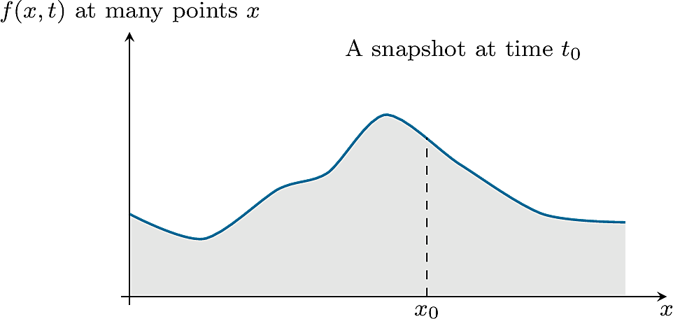
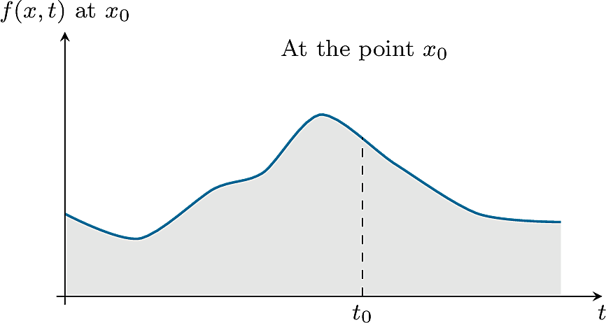
Let’s stop for a bit to ask what \(f(x,t)\) looks like. Since it depends on two variables, we can produce two types of plots1 as shown in Figure 1:
- If we fix \(t\), we get a snapshot in space of many particles at one instant.
- If we fix \(x\), we see how one particle moves in time.
3.3 Who Satisfies the Wave Equation?
If asked to think of a functional form for a wave, the first functions that might come to mind are trigonometric ones like \(\sin x\) or \(\cos x\). But a wave must involve both space and time. So, a more correct candidate is:
\[ f(x,t) = \sin(kx - \omega t) \]
where \(k\) and \(\omega\) are constants.
In fact, any function of the form \(f(kx - \omega t)\) is a wave: something that moves through space as time passes.
Here, \(f(kx - \omega t)\) is a general function that could represent, for example,
\(e^{kx - \omega t}\), \(\sin(kx - \omega t)\), \((kx - \omega t)^2\), and so on. By “function of the form,” I mean that \(x\) and \(t\) always appear together in the combination \(kx - \omega t\). Mathematically, \(f\) is just a function of \(x\) and \(t\). But since \(x\) and \(t\) always occur together with the signature \(kx - \omega t\), it is more insightful to write the function as \(f(kx - \omega t)\).
Now let me prove that \(f(kx - \omega t)\) is a wave using two approaches.
Brute force mathematical approach:
Let me show you that the function \(f(kx - \omega t)\) satisfies the wave equation.
Let \[ \theta \equiv kx - \omega t \]
so that \[ \frac{\partial \theta}{\partial x} = k, \qquad \frac{\partial \theta}{\partial t} = -\omega. \]
Let’s work on the variation in space. Here I will use the chain rulefor differentiation. \[ \frac{\partial f}{\partial x} = \frac{\partial f}{\partial \theta} \cdot \frac{\partial \theta}{\partial x} = k \frac{\partial f}{\partial \theta}. \]
Differentiating again: \[ \frac{\partial^2 f}{\partial x^2} = k \frac{\partial}{\partial x}\!\left(\frac{\partial f}{\partial \theta}\right) = k \frac{\partial}{\partial \theta}\!\left(\frac{\partial f}{\partial \theta}\right) \cdot \frac{\partial \theta}{\partial x} = k^2 \frac{\partial^2 f}{\partial \theta^2}. \]
So,
\[ \boxed{{\frac{\partial^2 f}{\partial \theta^2}=\frac{1}{k^2}\frac{\partial^2 f}{\partial x^2}} } \]
Now onto the differentiate with respect to \(t\):
\[ \frac{\partial f}{\partial t} = \frac{\partial f}{\partial \theta} \cdot \frac{\partial \theta}{\partial t} = -\omega \frac{\partial f}{\partial \theta}. \]
Differentiating again: \[ \frac{\partial^2 f}{\partial t^2} = -\omega \frac{\partial}{\partial t}\!\left(\frac{\partial f}{\partial \theta}\right) = -\omega \frac{\partial}{\partial \theta}\!\left(\frac{\partial f}{\partial \theta}\right) \cdot \frac{\partial \theta}{\partial t} = \omega^2 \frac{\partial^2 f}{\partial \theta^2}. \]
\[ \boxed{{\frac{\partial^2 f}{\partial \theta^2}=\frac{1}{\omega^2}\frac{\partial^2 f}{\partial t^2}} } \]
Comparing the boxed results, yields:
\[ \frac{1}{k^2}\frac{\partial^2 f}{\partial x^2} = \frac{1}{\omega^2}\frac{\partial^2 f}{\partial t^2}. \]
Or equivalently, \[ \frac{\partial^2 f}{\partial x^2} = \frac{1}{\left(\omega/k\right)^2}\frac{\partial^2 f}{\partial t^2}. \]
Comparing this with Equation 1, we see that any function of the form \(f(kx - \omega t)\) represents a wave. Further, the wave speed is given by:
\[ v = \frac{\omega}{k}. \tag{3}\]
Scrutinising the Form \(f(kx - \omega t)\)
A more elegant way to see that \(f(kx - \omega t)\) is a wave follows from looking closely at what this expression means.
Consider a snapshot of \(f\) at a time \(t_0 + \Delta t\). For the point at \(x=x_0\) the value if \(f\) is: \[ f\lrs{kx_0 - \omega (t_0 + \Delta t)} \]
But, \[ \begin{align} kx_0 - \omega (t_0 + \Delta t) &= kx_0 - \omega\Delta t -\omega t_0 \\ &= k(x_0 - \f{\omega}{k}\Delta t) -\omega t_0 \\ \underbrace{kx_0 - \omega (t_0 + \Delta t)}_\text{$f$ at $x_0$ at $(t_0 + \Delta t)$}&= \underbrace{kx' -\omega t_0}_\text{$f$ at $x'$ at $t_0 $} \\ \end{align} \]
Where, \(x'=x_0 - \f{\omega}{k}\Delta t\).
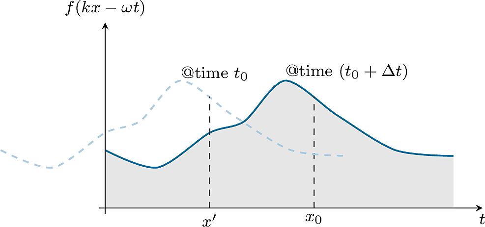
This tells us that the value of \(f\) at \((x_0, t_0 + \Delta t)\) is the same as the value at a shifted position \(x' = x_0 - \f{\omega}{k}\Delta t\) at an earlier time \(t_0\). In other words, the wave profile just shifts in the \(x\)-direction as time passes!
How fast does this shifting take place? The speed is simply:
\[ v = \f{\text{distance shifted}}{\text{time}} = \f{\f{\omega}{k}\Delta t}{\Delta t} = \f{\omega}{k} \]
4 Terminology
Let’s quickly remind ourselves of some terminology related to waves that we encounter often.
Imagine yourself floating in the ocean and experiencing the up-and-down motion as waves pass by. The highest points of the oscillation are called crests, and the lowest points are called troughs. The maximum displacement from the sea level is called the amplitude.
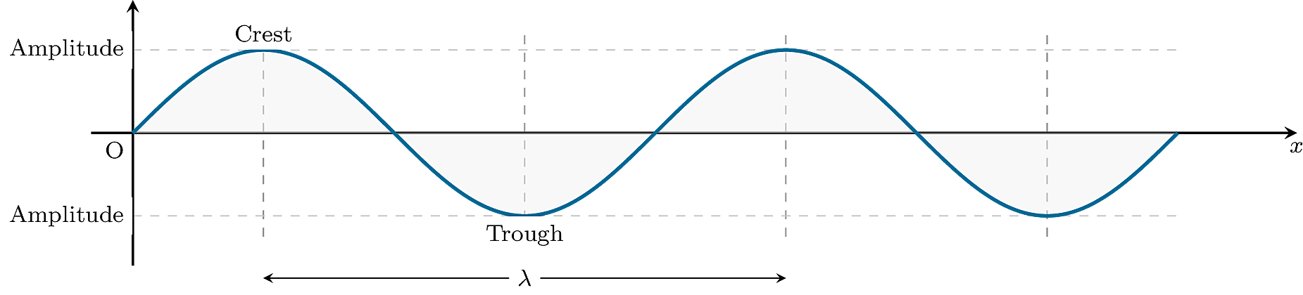
The number of times this up-and-down motion occurs in a given interval of time is related to the frequency. Specifically, the frequency \(f\) is the number of oscillations per second, measured in hertz (Hz). Closely related to this is the period \(T\), the time it takes to complete one oscillation. These quantities are connected through the relation
The distance between successive crests (or successive troughs) is called the wavelength \(\lambda\). Since a wave travels one wavelength \(\lambda\) in one period \(T\), the wave speed \(v\) is given by
\[ v = \frac{\lambda}{T} \]
Which leads us to the well-known relationship between the wave speed \(v\), the frequency \(f\), and the wavelength \(\lambda\):
4.1 What is \(k\) and \(\omega\)?
Let’s try to get a bit more insight into what \(k\) and \(\omega\) are.
Angular Wave Number \(k\)
First lets consider the function \(\cos kx\). What is its wavelength? To find this, we recall that the function must repeat after one wavelength \(\lambda\):
\[ \cos kx = \cos k(x + \lambda) = \cos kx + k\lambda . \]
This implies \[ k\lambda = 2\pi, \]
and consequently,
where \(k\) is called the angular wave number.
Angular Frequency \(\omega\)
Now consider \(\cos\omega t\). This function must repeat after one period \(T\) so: \[ \cos \omega t = \cos \omega (t + T) = \cos \omega t + \omega T . \]
This implies \[ \omega T = 2\pi, \]
and,
\[ \omega = \frac{2\pi}{T} \]
Since frequency is \(f = 1/T\),
where \(\omega\) is call the angular frequency.
4.2 The Ingredients for a Wave
Let’s pause for a bit to understand more clearly what it takes to generate a wave. I will use a wave in a medium as a general example. The only exception to this is light (electromagnetic waves), which does not require a medium and can propagate even through the vast emptiness between stars. For the moment, however, you can imagine that there is always a medium. This makes it easier to visualise how waves behave, without immediately having to grapple with the more abstract ideas required for electromagnetic waves.
At its core, a wave is simply a way of passing on a disturbance that is caused by a source. The source disturbs the medium by imparting energy into the medium, and a restoring force acts to bring the medium back to its original state. How strongly this restoring force acts will influence how the disturbance propagates. The nature of the medium (e.g. density, rigidity) then determines how fast the wave can travel.
So, a wave requires:
- A source of energy (to generate the disturbance).
- A medium or mechanism (that can ‘hold’ the energy transferred by the source),
- A restoring force (to push the medium back).
The wave is therefore a consequence of the system trying to restore itself to its equilibrium state. A wave is simply the disturbance being passed along from one connected part of the medium to the next.
The table below shows some typical waves we encounter.
| Wave | Restoring Force | Medium Parameter of Importance |
|---|---|---|
| Ocean (gravity) waves | Gravity | \(\rho\) density of water |
| Guitar String | Tension | \(\mu\) mass per unit length |
| Sound waves | Intermolecular attraction | \(\rho\) density of medium |
| Electromagnetic (EM) | Maxwell’s equations(electric and magnetic fields restoring each other) | \(\varepsilon_0\), \(\mu_0\) properties of vacuum |
4.3 Energy Stored in a Wave
The energy stored in a wave is ultimately stored in how the disturbance distorts the medium.
- In a water wave, energy is stored as the kinetic and gravitational potential energy of the particles.
- In a sound wave, energy is also stored as kinetic and elastic potential energy of the medium.
- Light is very special: it is made up of oscillating electric and magnetic fields, and these fields themselves store energy simply by existing!
Since a wave is about transferring energy, it makes more sense to talk about how much energy flows past in a given time. This leads to the idea of intensity.
However, due to the oscillatory nature of waves, the instantaneous intensity at any point changes with time. It therefore makes sense to also talk about the average intensity over time. I will denote this time average as \(\langle I \rangle\). To get a feel of what we are dealing with the table below shows the average intensities for several different waves.
| Wave | Average Intensity \(\langle I \rangle\) | Notes |
|---|---|---|
| Ocean (gravity) waves | \(\f{1}{2}\,\rho g A^2 v\) | \(\rho\) density of water, \(g\) gravity, \(v\) wave speed, \(A\) amplitude |
| Guitar string | \(\f{1}{2}\,\mu \omega^2 A^2 v\) | \(\mu\) mass per unit length of string, \(v\) wave speed, \(A\) amplitude |
| Sound wave | \(\f{1}{2}\,\rho v \omega^2 s_0^2\) | \(\rho\) medium density, \(v\) sound speed, \(s_0\) displacement amplitude |
| Electromagnetic (EM) | \(\f{1}{\mu_0} E_0 B_0 = \tfrac{1}{2} c \varepsilon_0 E_0^2\) | \(\mu_0\) permeability of free space, \(\varepsilon_0\) permittivity of free space, \(c\) speed of light, \(E_0\) electric field amplitude |
Although the exact form of the expressions differs from one type of wave to another, you will notice a common pattern: the average intensity always depends on the square of the amplitude, the square of the frequency, and the speed of the wave.
4.4 Dispersion and Wave Speed
4.5 Wave Speeds
How fast a wave travels in a medium depends on how the medium responds to deformation. To give you a feel for how this works out the table below gives the expressions for the speed of different waves.
| Wave | Wave Speed \(v\) | Notes |
|---|---|---|
| Ocean (gravity) waves | \(\begin{align*}v &= \sqrt{gd}\quad\text{(shallow water)}\\v &= \sqrt{\dfrac{g \lambda}{2\pi}}\quad\text{(deep water, $d \gt \frac{1}{2}\lambda$)}\end{align*}\) | \(d\) depth \(g\) gravity, \(\lambda\) wavelength |
| Guitar string | \(v = \sqrt{\dfrac{T}{\mu}}\) | \(T\) tension in string, \(\mu\) mass per unit length |
| Sound wave | \(v = \sqrt{\dfrac{B}{\rho}}\) | \(B\) bulk modulus (compressibility), \(\rho\) density |
| Electromagnetic (EM) | \(c = \f{1}{\sqrt{\mu_0 \varepsilon_0}}\) | \(\mu\) permeability, \(\varepsilon\) permittivity |
5 Superposition of Waves & Interference
When waves add up according to the principle of superposition, we say that they are interfering. Interference is one of the most fundamental features of waves. In fact, almost all other wave-related phenomena (such as reflection, refraction, and diffraction) can ultimately be traced back to interference.
Consider two waves:
\[\begin{align} f_1 &= A \cos(kx - \omega t)\\ f_2 &= A \cos(kx - \omega t + \alpha) \end{align}\]
where \(A\) is the amplitude and \(\alpha\) is a constant called the phase difference between the waves (we will return to the idea of phase difference in more detail soon).
If these waves interfere along the \(x\)-axis: \[ f = f_1 + f_2 = 2A \cos \lr{\f{\alpha}{2}}\cos \lr{kx - \omega t + \f{\alpha}{2}} \]
Since we are interested in superposition at a given point in space, we can safely examine the displacements at a fixed time \(t = 0\) without losing generality.
\[ f = f_1 + f_2 = 2A \cos \lr{\f{\alpha}{2}}\cos \lr{kx + \f{\alpha}{2}} \]
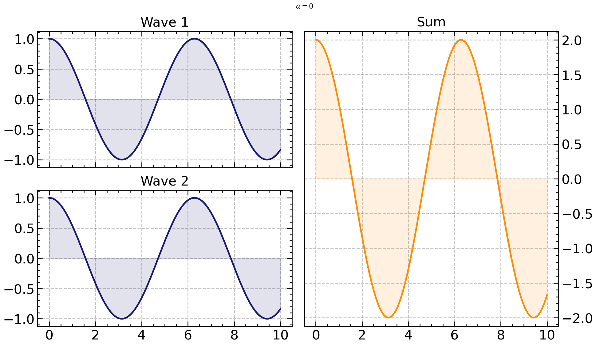
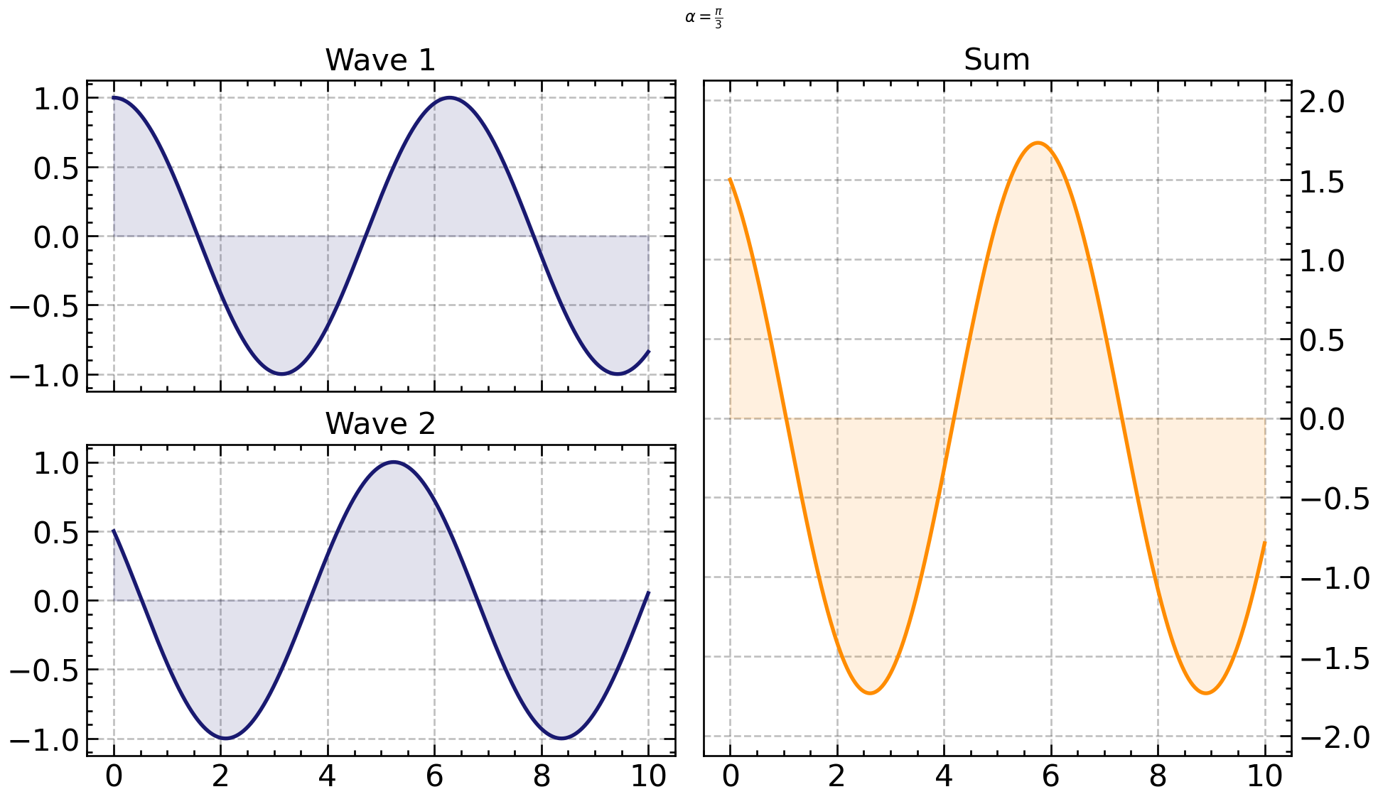
Different values of \(\alpha\) determine the way in which the two waves interfere. Let’s plot this with \(\lambda=1\) for different values of \(\alpha\).
\(\alpha = 0\) so the waves are in complete agreement and add up maximally.
\(\alpha = \pi\) so the waves are in complete disagreement and cancel each other out.
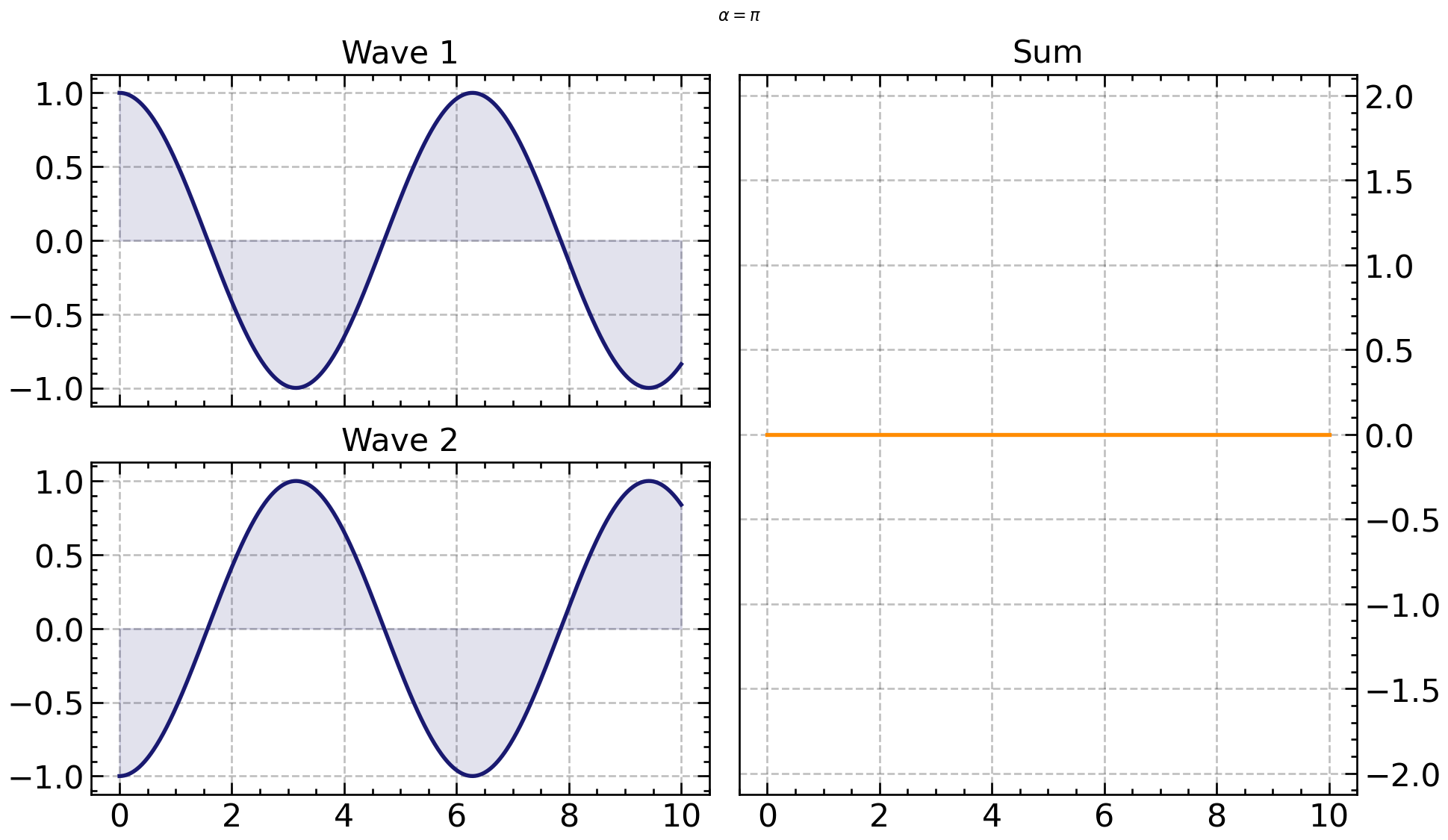
\(0 < \alpha < \pi\) so this is a state between constructive and destructive interference is called partial interference. In this case, the resulting amplitude lies between the two extremes.
6 Fundamental Wave Phenomena
There are three2 other fundamental wave phenomena (besides interference) that I want to highlight: Reflection, Refraction, and Diffraction.
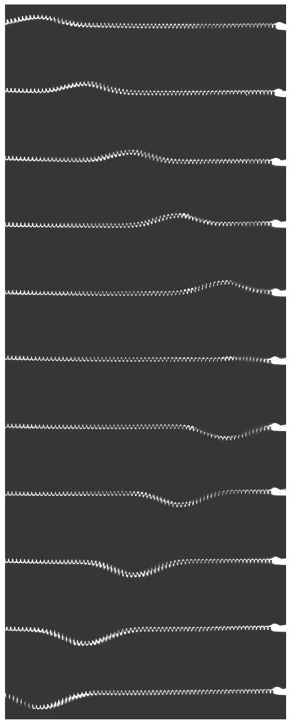
Reflection is the bouncing of waves off an obstacle. You can see this in Figure 5 alongside.
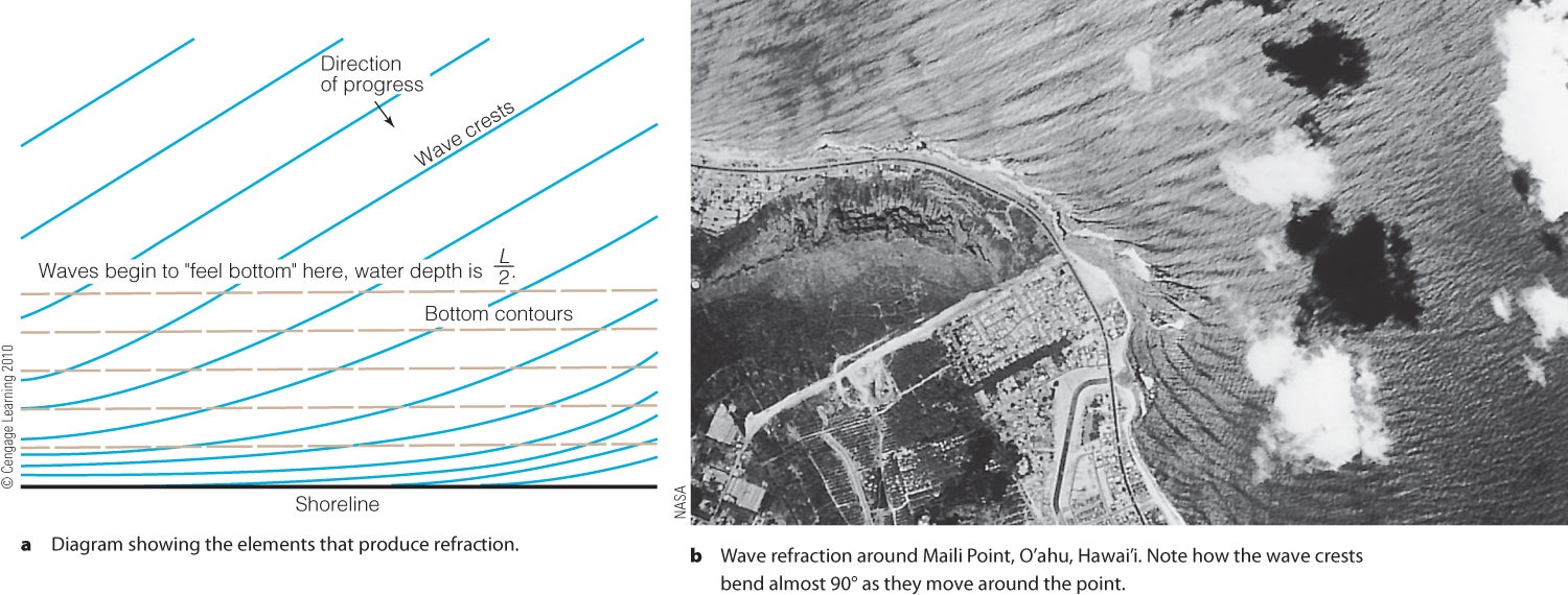
Refraction is the bending of waves at a boundary due to a change in speed, as shown in Figure 3.
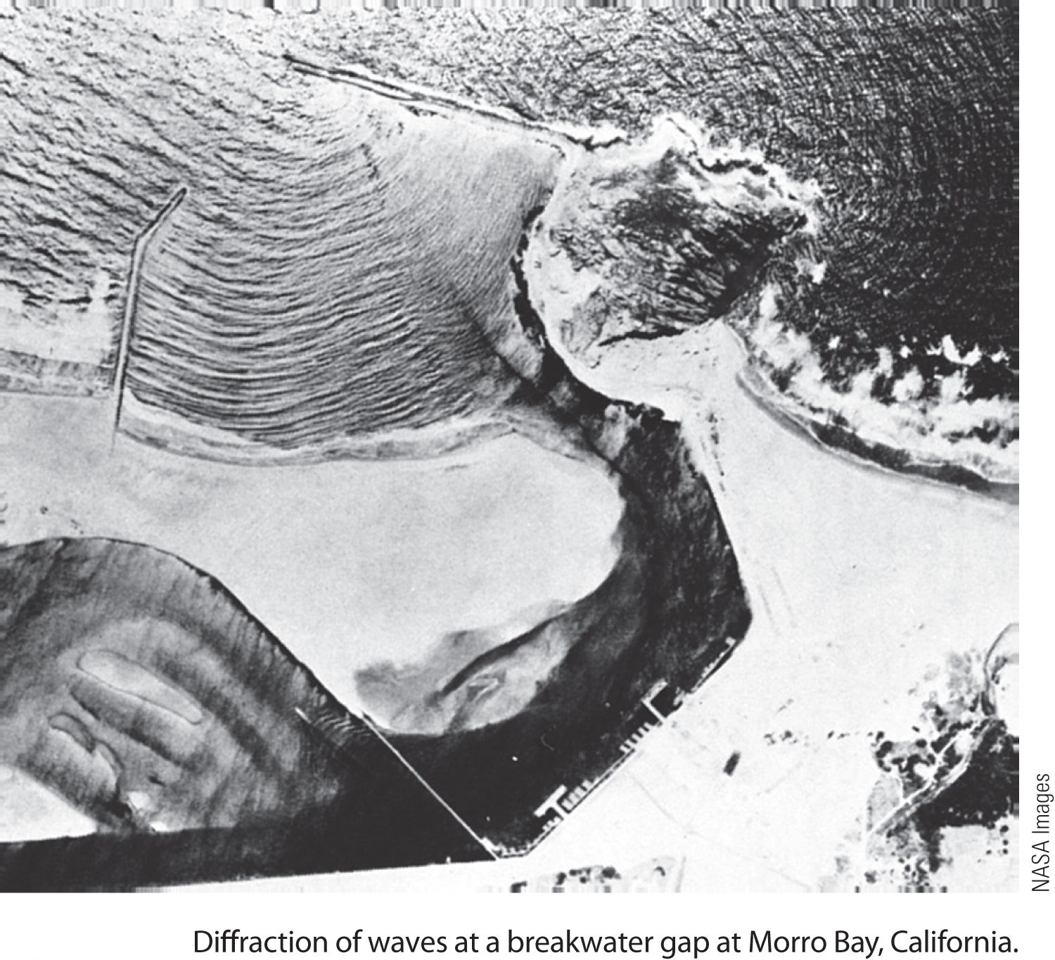
Diffraction is the bending of a wave when it passes through a gap or around an obstacle, as in Figure 4. The degree of bending depends on how the size of the gap or obstacle compares with the wavelength.
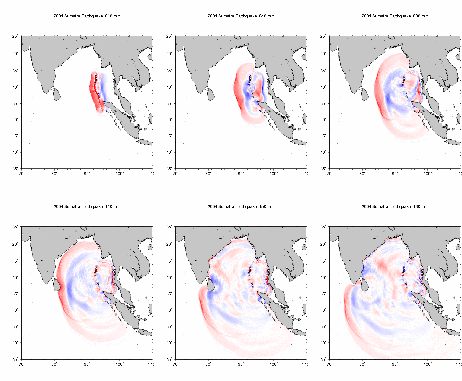
For example, we can hear people talking around a corner because of sound diffraction. Another striking example is a tsunami. Being waves, tsunamis also exhibit diffraction. Figure 6 shows a simulation of the 2004 Indian Ocean tsunami: notice how the wave bends around Sri Lanka and impacts cities on the western side of the island.
7 Path Difference & Phase Difference
7.1 The Idea of Path and Phase Difference
Consider two waves that occupy the same space so that they end up interfering. We know from the section of superposition that the result of this interference depends on the alignment of their crests (or troughs). We use the terms phase difference and path difference to describe this alignment. Knowing the phase or path difference between waves is crucial to predicting how they will interfere.
Both phase difference (\(\phi\)) and path difference (\(\Delta\)) describe the same property related to alignment but in different units:
- \(\phi\) is an angle (measured in radians).
- \(\Delta\) is a length (measured in metres).
These are related by: \[ \phi \;=\; 2\pi\lr{\f{\Delta}{\lambda}} \tag{8}\]
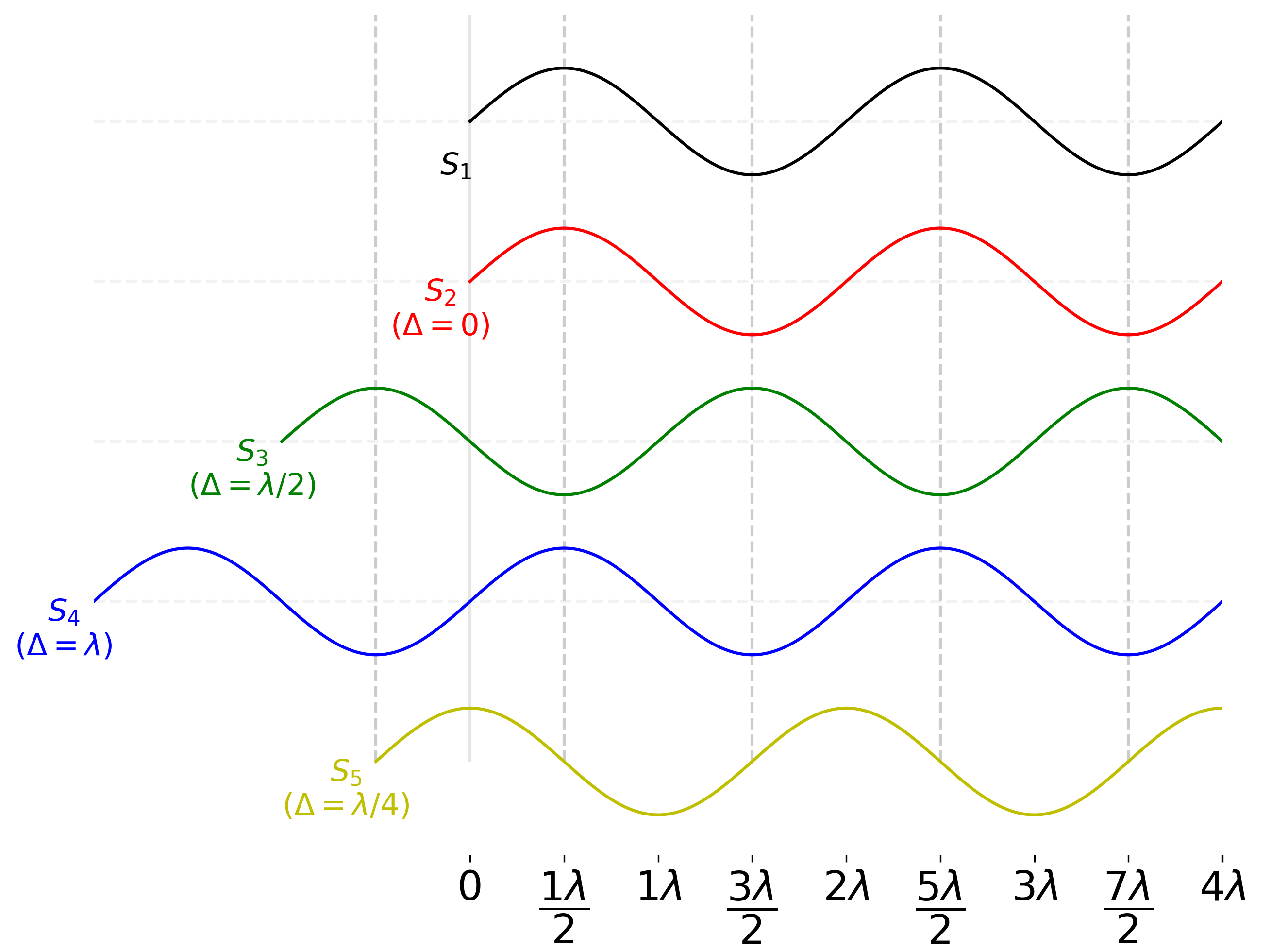
Figure Figure 7 illustrates the idea of \(\phi\) and \(\Delta\). It shows five identical sources placed at different locations along a straight line (separated vertically for clarity). The path difference is measured with respect to source \(S_1\).
| Path Difference (\(\Delta\)) |
Phase Difference (\(\phi\)) |
Type of Interference |
|---|---|---|
| \(n\lambda\) (Even multiple of \(\lambda\)) |
\(2n\pi\) (Even multiple of \(\pi\)) |
Constructive |
| \((2n+1)\f{\lambda}{2}\) (Odd multiple of \(\f{\lambda}{2}\)) |
\((2n+1)\pi\) (Odd multiple of \(\pi\)) |
Destructive |
7.2 Phase Due to Reflection
If you take a look at Figure 5, you will notice that the reflected wave undergoes a \(\pi\) phase flip. This behaviour is universal for waves reflecting off a denser medium (where the wave speed is slower).
- The adjoining video which demonstrates both these behaviours.
- This seemingly simple characteristic is extremely important for using waves (especially light) for interferometry as you would see during project 1.
Footnotes
Plotting in 3D is a terrible, terrible idea. See Fundamentals of Data Visualization↩︎
Actually four; the fourth is polarisation, which applies only to transverse waves. We’re listing three here because we’re treating interference separately.↩︎