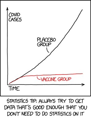
Statistics is wonderfully practical, and almost everyone can benefit from learning its basic ideas. Although statistical tools can be used as black boxes, it is worth understanding what their results actually mean. Statistics is one of those subjects where a little knowledge, applied uncritically, can quickly become misleading, or even embarrassing.
Before proceeding, I must say that no amount of sophisticated analysis can compensate for poor data collection. A statistical result is only as meaningful as the measurement process that produced the data. In particular, a small statistical uncertainty does not guarantee an accurate result: measurements can be precise yet systematically biased.
Imagine that we could repeat an experiment indefinitely under identical conditions. The collection(distribution) of all possible outcomes is called the population distribution or parent distribution.
In reality, we can make only a finite number of measurements. These measurements form a sample, which we use to learn about the underlying population.
The purpose of statistical inference is to use a sample to learn about the population:
sample \(\quad\Longrightarrow\quad\) population.
2 Mean
For a sample containing the measurements \(x_1,x_2,x_3,\ldots,x_N,\) the sample mean, or average, is: \[
\bar{x}=\frac{1}{N}\sum_{i=1}^{N}x_i.
\tag{1}\]
An important result concerning the sample mean is the Law of Large Numbers.
ImportantLaw of Large Numbers (LLN)
As the sample size increases, the sample mean tends to approach the population mean.
What does this mean for an experiment?
We often use the mean as a representative value for repeated measurements. This relies on the idea that the errors/uncertainties associated with the measurement process are random so that with enough measurements, the positive and negative deviations tend to cancel out. Systematic bias, however, does not disappear through repetition.
How many trials should be carried out?: According to the Law of Large Numbers, collecting more measurements generally improves our estimate of the population mean. However, “take as many measurements as possible” ignores experimental realities. Time, instrument limitations, changing conditions, and other practical constraints get in the way, as we will soon see with the pendulum.
The corresponding mean of the parent population is usually denoted by \(\mu\).
3 Standard deviation
The sample standard deviation, denoted by \(s_x\), describes how widely the measurements are spread around the sample mean \(\bar{x}\):
We use \(s_x\) to estimate the standard deviation of the parent population from a finite sample of \(N\) measurements.
We divide by \(N-1\), rather than \(N\), because the population mean is unknown and has been estimated using the sample mean \(\bar{x}\)1. This distinction between \(N\) and \(N-1\) matters most for small samples. For large \(N\), the difference becomes negligible.
How large a sample is “large enough” depends on the experiment, the natural variation in the measurements, and the precision we require. Collecting more data generally improves an estimate, but within reason as we will see in a bit.
The corresponding standard deviation of the parent population is usually denoted by \(\sigma\).
The standard deviation describes the variation among individual measurements. It is different from the uncertainty associated with the sample mean, which is quantified by the standard error.
4 Distributions
A probability distribution provides a framework for answering questions about patterns, frequencies, and expectations across repeated events or measurements. It helps us connect mathematical models with experimental data and develop a statistical understanding of the system we are studying.
There are many probability distributions, including the normal, Student’s \(t\), Poisson, chi-square, and Cauchy distributions. Identifying an appropriate distribution can make data analysis much easier, provided that its assumptions are reasonable for the process being studied.
4.1 Three important distributions
Let me highlight three distributions that you will encounter frequently in this course and beyond.
Normal or Gaussian distribution
The normal distribution is the familiar symmetric, bell-shaped distribution. It is described by two parameters:
the mean \(\mu\), which sets its centre;
the standard deviation \(\sigma\), which sets its spread.
If a variable is normally distributed, approximately:
68% of its values lie within \(\mu\pm\sigma\);
95% lie within \(\mu\pm2\sigma\);
99.7% lie within \(\mu\pm3\sigma\).
This is sometimes called the 68–95–99.7 rule.
Figure 2: The 68–95–99.7 rule for Normal distributions. (Source: Wikipedia)
The normal distribution appears frequently in measurement science because the combined effect of many small, independent sources of variation often produces an approximately normal distribution.
Student’s \(t\)-distribution
Student’s \(t\)-distribution resembles the normal distribution but has heavier (longer) tails. Its shape depends on the number of degrees of freedom, denoted by \(\nu\).
For a sample of size \(N\) used to estimate a mean,
\[
\nu=N-1.
\]
The \(t\)-distribution approaches the normal distribution as the sample size, and hence \(\nu\), increases.
The heavier tails of the \(t\)-distribution accounts for the additional uncertainty introduced by replacing \(\sigma\) with the sample standard deviation \(s\). This correction is most important for small samples with fewer than 30 observations.
Figure 3: Normal vs. Student’s \(t\) distribution. (Image source)
We will use the \(t\)-distribution when constructing confidence intervals for a population mean from experimental data.
Poisson distribution
For a counting experiment, where
events occur independently of one another;
events occur at an approximately constant average rate;
the distribution of data follows the Poisson distribution.
The Poisson distribution is a discrete probability distribution that describes the number of events observed within a fixed interval of time, distance, area, or volume.
For example:
the number of particles detected in one second,
the number of cells observed in a grid square,
the number of seagrass plants within a quadrat,
the number of radioactive decays recorded during a fixed time interval,
the number of babies born in a hospital during a week.
Figure 4: The Poisson Distribution
A Poisson distribution is described by a single parameter, \(\lambda\), which is both the expected number of events in the chosen interval and the population mean \(\mu\).
As \(\lambda\) becomes large, the Poisson distribution becomes increasingly symmetric and can be approximated by a normal distribution with
5 Standard error (SDOM)
We typically use the mean (\(\bar{x}\)) of repeated measurements or trials (\(x_1, x_2, x_3,\ldots,x_N\)) as our best estimate of the quantity being measured.
The standard deviation, \(s_x\), describes the variation among the individual measurements (i.e. \(x_1, x_2, x_3,\ldots,x_N\)). The standard error describes the uncertainty associated with the sample mean (\(\bar{x}\)) we calculate from the individual trials. This standard error is given by: \[
s_{\bar{x}}=\frac{s_x}{\sqrt{N}},
\tag{3}\]
where \(N\) is the number of trials.
This means that increasing the number of trials improves the precision of the mean but with diminishing returns; to halve the standard error, we need four times as many measurements.
We can report an experimental result as:
\[
x=\bar{x}\pm\frac{s_x}{\sqrt{N}}.
\tag{4}\]
This gives the mean with one standard error.
The theory behind the standard error related to the following important theorem in statistics:
ImportantCentral Limit Theorem
The distribution of sample means is a Gaussian with standard deviation \[
s_{\bar{x}} = \frac{s_x}{\sqrt{N}}
\tag{5}\]
Note: We create the distribution of sample means above by repeating the entire experiment many times, with each experiment containing \(N\) trials.
For this reason, the standard error is also called the standard deviation of the mean (SDOM).
6 The error of the error
The standard error is estimated from a finite sample and therefore has its own uncertainty: the error of the error. So, this brings us to an important question: how precisely do we know the standard error itself? Should we report it using one, two, or three significant figures?
This matters a lot because the uncertainty determines how we round and report the measured value. For small samples, the standard error is known precisely enough to justify quoting many significant figures. So, as a practical rule:
ImportantError of the error
Quote the uncertainty to one significant figure, and round the measured value to the same decimal place.
The following example, adapted from1, illustrates this nicely:
Example 1 (Importance of the error-of-error)
Suppose two experiments, each based on \(N=10\) repeated measurements, produce the following results:
Mean, \(\bar{x}\)
SDOM, \(s_{\bar{x}}\)
How to report the result
\(9.8123456\)
\(0.0321987\)
\(x=(9.81\pm0.03)\)
\(9.817654\)
\(0.10123\)
\(x=(9.8\pm0.1)\)
6.1 What about NIST?
If you visit NIST and look up the electron mass, you will find
NIST can report this level of precision because CODATA values are obtained through a combination of highly precise measurements, theoretical relationships, and correlations between different quantities. It involves more than simply repeating one experiment a very large number of times.
7 Confidence intervals
Earlier, we discussed how the standard error (\(s_{\bar{x}}\)) describes the precision of a sample mean. We can express this information more meaningfully by constructing a range around the mean that expresses the confidence in the measurement.
For a sufficiently large sample, an approximate 95% confidence interval is
\[
\bar{x}\pm1.96s_{\bar{x}}.
\]
This range is called a 95% confidence interval (CI).
For smaller samples, it is more accurate to use Student’s \(t\)-distribution:
\[
\bar{x}\pm t^*\frac{s_x}{\sqrt{N}},
\]
where \(t^*\) depends on the sample size and can be calculated using Python (see the example below).
A 95% confidence interval would contain the population mean in approximately 95% of repeated experiments. It does not mean that 95% of the individual measurements lie within the interval.
Example 2 (Determining the CI for set of data)
import numpy as npfrom scipy.stats import t# Some dummy dataperiods = np.array([2.010, 2.006, 2.008, 2.012, 2.007])# Sample statisticsn =len(periods)mean = np.mean(periods)s = np.std(periods, ddof=1) # Use ddof=1 for Sample std. dev.standard_error = s / np.sqrt(n)# Critical value for a 95% confidence interval using Student's tcritical_value = t.ppf(0.975, df=n -1)# Confidence intervalmargin = critical_value * standard_errorci = (mean - margin, mean + margin)print(f"Mean = {mean:.4f} s")print(f"Standard deviation = {s:.4f} s")print(f"Standard error = {standard_error:.4f} s")print(f"95% CI = ({ci[0]:.4f}, {ci[1]:.4f}) s")
Mean = 2.0086 s
Standard deviation = 0.0024 s
Standard error = 0.0011 s
95% CI = (2.0056, 2.0116) s
8 Some consequence for Activity I
Let me now use the above ideas to in the context of the experiment you have to play with.
8.1 How many oscillations should be measured?
First, timing more than one oscillation can reduce the effect of start and stop timing errors. If the total timing uncertainty is approximately \(u_{t_N}\), then \[
u_T=\frac{u_{t_N}}{N}.
\]
For example, a timing error of \(0.2\) s has a much larger effect when divided by one oscillation than when divided by twenty oscillations.
However, increasing \(N\) does not solve every problem. A longer timing interval can introduce other effects:
the amplitude may decrease noticeably;
the bob may drift out of its intended plane;
the counter may lose track of the oscillations; or
the apparatus may be disturbed.
So, the decision boild down to a trade-off in the experimental design. The useful question is therefore not:
“What is the largest possible \(N\)?”
but:
“What value of \(N\) reduces important timing effects without allowing other effects to dominate?”
8.2 How many repeated measurements are needed?
There is no universal correct number of repeats. The required number depends on:
the spread of individual measurements;
the smallest difference worth detecting;
the desired confidence level;
the cost or time of each measurement; and
whether the measurement method is stable.
However, once we have a pilot dataset, it can provide an initial estimate of the spread. If the desired uncertainty in a mean is \(E\), a rough planning estimate is \[
N\approx\left(\frac{z s}{E}\right)^2,
\]
where \(z\) is approximately (\(\approx 1.96\)) 2 for a rough 95% target based on a Normal distribution.
If the aim is to detect a difference \(\delta\) between two independent groups with similar spread \(s\), a rough estimate for the number of measurements per group is
\[
n\approx2\left(\frac{z s}{\delta}\right)^2.
\]
These equations are planning approximations, not guarantees. They assume that the measurements are reasonably independent and that the pilot spread is representative.
For the pendulum activity, a sensible strategy is:
collect a small pilot dataset;
estimate the spread;
identify the smallest difference that would matter physically;
decide whether the current precision is adequate; and
collect more measurements or improve the method if needed.