f = 14.0 ± 0.9Experimental Uncertainties
Activity 1 | Week 1 | Background Material
“Any measurement that you make without the knowledge of its uncertainty is completely meaningless”
– Walter Lewin.
1 Uncertainties and errors in measurements
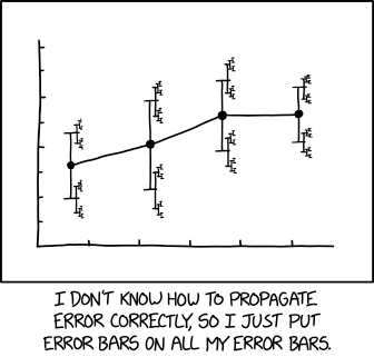
When we repeat the same measurement many times, we almost never get exactly the same value each time. Instead, the results spread out. This makes it tricky to decide on a single `true’ value. Every experimental result therefore has some associated uncertainty, and reporting this uncertainty is as important as reporting the measurement itself. A numerical result may mean very little if its uncertainty is unknown or unacceptably large.
The terms measurement error and measurement uncertainty are sometimes used interchangeably, but they have different meanings:
- Measurement error is the difference between a measured value and the true value, which is usually unknown.
- Measurement uncertainty quantifies how well the measured result is known. It combines the relevant effects into a quantitative statement of how well the measured result is known.
Uncertainty and error can arise from several sources:
| Source | Meaning | Typical response |
|---|---|---|
| Random variation | Unpredictable trial-to-trial variation | Repeat measurements and quantify the spread |
| Systematic bias | A consistent shift away from the true value | Calibrate, improve, or redesign the method |
| Instrument resolution | The smallest change the instrument can detect | Include the resolution in the uncertainty |
| Procedural variation | Changes in release, alignment, timing, or observation | Standardize the procedure |
| Environmental variation | Changes in temperature, vibration, airflow, or other conditions | Monitor or control the environment |
| Invalid measurement | A known failure of the intended procedure | Record the reason, exclude it transparently, and repeat the measurement |
I like to point out that a measurement can be precise but biased.
For example:
- a timer that runs consistently slow may produce very similar results in every trial while systematically underestimating the true period. Repeating the measurement can reduce the random uncertainty in the mean, but it will not remove the bias.
- Repeated measurements that give the same value are not necessarily free from uncertainty. An instrument with limited resolution may repeatedly display the same reading even though the true value remains uncertain.
2 Significant figures and decimal places
2.1 Significant figures
This is a good place to talk briefly about numbers in measurements. The number of digits reported should reflect the precision of the measurement you have made. Extra digits that appear when you perform calculations do not make the result more accurate and usually have no physical meaning.
Let us say that you measure the diameter of a tin as \(10.3\ \mathrm{cm}\).
- You could write the diameter as \(103\,000\ \mu\mathrm{m}\). However, you have gained no additional information by changing the units. The final three zeros do not represent greater precision: they are not significant.
- You could also write the same measurement as \(0.103\ \mathrm{m}\). Here, the zero between 1 and 3 is significant, while the zero before the decimal point is not.
In all three cases, the measurement has three significant figures.
Identifying significant figures
Here are the basic rules for identifying significant figures. All the numbers in Table 2, except the last one, have four significant figures.
| Example | Rule |
|---|---|
| \(\;1.234\) | All non-zero digits are significant. |
| \(\;1.023\) | Zeros between non-zero digits are significant. |
| \(0.1234\) | Zeros before the first non-zero digit are not significant. |
| \(\;1.600\) | Trailing zeros after a decimal point are significant. |
| \(\;2700\) | Trailing zeros without a decimal point are ambiguous. |
The final example could represent two, three, or four significant figures. Using scientific notation removes the ambiguity:
- Write \(2.7\times10^3\) to indicate 2 significant figures.
- Write \(2.70\times10^3\) to indicate 3 significant figures.
- Write \(2.700\times10^3\) to indicate 4 significant figures.
Writing \(2700.\) can also indicate 4 significant figures, but scientific notation is clearer.
How to round significant figures
Here are the rules for rounding to a specified number of significant figures. In Table 3, we are rounding each number to two significant figures by retaining the first digit after the decimal point.
| Example | Next digit | Rule |
|---|---|---|
| \(6.62\) becomes \(6.6\) | 0–4 | Leave the last retained digit unchanged. |
| \(5.67\) becomes \(5.7\) | 6–9 | Increase the last retained digit by 1. |
| \(3.45\) becomes \(3.4\) | 5 and the retained digit is even | Leave the retained digit unchanged. |
| \(3.55\) becomes \(3.6\) | 5 and the retained digit is odd | Increase the retained digit by 1. |
The rules for handling an exact 5 are known as the round-to-even method. This method applies when 5 is the final digit.
2.2 Errors from instruments
I have pinched the following from
- The precision of an analogue device is half of the smallest division of the instrument.
- The precision of a digital device is one in the last digit displayed.
- The precision of a measurement is only equal to the precision of the measuring device if repeat measurements are identical.
3 How to propagate uncertainty
In experiments, we are rarely able to measure the exact quantity we are interested in. More often than not, we measure related parameters and then infer the desired value. This is where the idea of error propagation becomes important: we must propagate the uncertainties of our measured quantities to the final result.
The traditional way of carrying out error propagation can be laborious. It involves calculating partial derivatives of the function with respect to each variable and then adding the contributions in quadrature.
Fortunately, there are easier alternatives. In this section,we will focus on three approaches.
3.1 Option 1:Simple uncertainty-propagation formulae
Let \(u_x\), \(u_y\), and \(u_z\) denote the standard uncertainties in \(x\), \(y\), and \(z\).
| Operation | Relationship | Propagated uncertainty |
|---|---|---|
| Constant multiple | \(z=ax\) | \(u_z=|a|u_x\) |
| Addition or subtraction | \(z=x\pm y\) | \(u_z=\sqrt{u_x^2+u_y^2}\) |
| Multiplication | \(z=xy\) | \(\displaystyle \frac{u_z}{|z|}=\sqrt{\left(\frac{u_x}{x}\right)^2+\left(\frac{u_y}{y}\right)^2}\) |
| Division | \(\displaystyle z=\frac{x}{y}\) | \(\displaystyle \frac{u_z}{|z|}=\sqrt{\left(\frac{u_x}{x}\right)^2+\left(\frac{u_y}{y}\right)^2}\) |
| Power | \(z=x^n\) | \(\displaystyle u_z=|nx^{n-1}|u_x\) |
| Sine | \(z=\sin x\) | \(u_z=|\cos x|u_x\) |
| Inverse sine | \(z=\sin^{-1}x\) | \(\displaystyle u_z=\frac{u_x}{\sqrt{1-x^2}}\) |
| Cosine | \(z=\cos x\) | \(u_z=|\sin x|u_x\) |
| Inverse cosine | \(z=\cos^{-1}x\) | \(\displaystyle u_z=\frac{u_x}{\sqrt{1-x^2}}\) |
| General function | \(z=f(x)\) | \(\displaystyle u_z=\left|\frac{df}{dx}\right|u_x\) |
| General multivariable function | \(z=f(x,y,\ldots)\) | \(\displaystyle u_z=\sqrt{\left(\frac{\partial f}{\partial x}u_x\right)^2+\left(\frac{\partial f}{\partial y}u_y\right)^2+\cdots}\) |
Please note:
- These formulae assume that the uncertainties are small and that the input quantities are independent.
- For trigonometric functions, angles and their uncertainties must be expressed in radians. The uncertainty in \(\sin^{-1}x\) becomes very large as \(x\) approaches \(-1\) or \(1\).
Example 1 (Using error propagation formuale)
Consider a hypothetical experiment where we measure \(x\) and \(y\) in order to determine \(f\) through the relationship \[ f(x,y) = x + y^2 . \]
Our measurements are:
| \(\bar{x} = 10.0\) | \(s_x = 0.5\) |
| \(\bar{y} = 2.0\) | \(s_y = 0.2\) |
Based on Table 4:
\[\begin{align} u_f^2 &= [1]^2\,u_x^2 + [2y^{(2-1)}]^2\,u_y^2 \\ &= u_x^2 + 4y^2u_y^2 \\ &= (0.5)^2 + 4(2)^2(0.2)^2 \\ &= 0.89 \end{align}\]
Whence, \(u_f = 0.9\) and we will report our result as \(f=14.0 \pm 0.9\)
Let me now show you another example that highlights the value of uncertainty propagation. In this case, it allows us to compare two methods of measuring an angle.
Example 2 (Two methods to measure angle) Suppose that we want to measure an angle of approximately \(10^\circ\). We have two possible methods:
- Use a protractor with a minimum division of \(1^\circ\).
- Measure the sides of a right-angled triangle using a ruler with a minimum division of \(1\) mm(\(=0.1\) cm), and then calculate the angle.
Which method gives the more precise result?
Suppose that the measured angle is \(\theta=10^\circ\) with an uncertainty of: \[ u_\theta=1^\circ. \]
The relative uncertainty is therefore: \[ \frac{u_\theta}{\theta} = \frac{1^\circ}{10^\circ} = 0.10 (=10\%). \]
We would report the result as
\[ \theta=(10\pm1)^\circ. \]
Suppose that we construct a right-angled triangle and measure:
- \(a=(17.4\pm0.1)\ \mathrm{cm}\) for the opposite side, and
- \(b=(100.0\pm0.1)\ \mathrm{cm}\) for the hypotenuse.
First, taking, \(z=\dfrac{a}{b}\), leads to an uncertainty in \(z\) of \[ \frac{u_z}{z} = \sqrt{ \left(\frac{u_a}{a}\right)^2+ \left(\frac{u_b}{b}\right)^2 }. \] Therefore, \[ z=\frac{17.4}{100.0}=0.174 \qquad \text{and} \qquad u_z = z \sqrt{ \left(\frac{0.1}{17.4}\right)^2+ \left(\frac{0.1}{100.0}\right)^2 } \approx0.0010. \]
The angle is \(\theta\) is given by:
\[ \sin \theta = \dfrac{b}{a}=z \quad\Rightarrow \quad\theta=\sin^{-1}(z)\approx10.0^\circ. \]
The uncertainty inverse sine is obtained using,
\[ u_\theta = \frac{u_z}{\sqrt{1-z^2}}. \]
Let’s remember that we must use radians and evaluate: \[ u_\theta \approx \frac{0.0010}{\sqrt{1-0.174^2}} \approx0.0010\ \mathrm{rad} \approx0.06^\circ (= 0.6\%). \]
We would therefore report \[ \theta=(10.0\pm0.06)^\circ. \]
- Notice how significantly (over two orders of magnitude!) more precise this method is.
- Even if you were sloppy and measured the lengths with an uncertainty of 0.5 cm, this method will still yield a superior (\(u_\theta \approx 3\%\)) measurement of the angle!
- There are other issues that we haven’t accounted for such as: an imperfect right angle or difficulty identifying the ends of the triangle. These add more uncertainty.
3.2 Using a Python package
You can also use a suitable Python package such uncertainties
Here is hpw to use uncer for the two previous examples:
Example 3
Example 4
import numpy as np
from uncertainties import ufloat
from uncertainties.umath import asin

# Lengths in centimetres
a = ufloat(17.4, 0.1)   # Opposite side
b = ufloat(100.0, 0.1)  # Hypotenuse

theta_rad = asin(a / b)

# Convert radians to degrees
theta_deg = theta_rad * 180 / np.pi

print(
    f"θ = {theta_deg.nominal_value:.2f} "
    f"± {theta_deg.std_dev:.2f}°"
)
θ = 10.02 ± 0.06°4 A worked example
import numpy as np
from scipy.stats import t

T10 = np.array([2.010, 2.006, 2.008, 2.012, 2.007])
T20 = np.array([2.019, 2.017, 2.021, 2.018, 2.020])
n = len(T10)


def summarize(data):
    mean = np.mean(data)
    s = np.std(data, ddof=1)  # Sample standard deviation
    u_mean = s / np.sqrt(len(data))
    return mean, s, u_mean


mean10, s10, u10 = summarize(T10)
mean20, s20, u20 = summarize(T20)

delta = mean20 - mean10
u_delta = np.sqrt(u10**2 + u20**2)

# Critical value from Student's t-distribution
critical_value = t.ppf(0.975, df=n-1)  # 2.5% in each tail

ci = (
    delta - critical_value * u_delta,
    delta + critical_value * u_delta,
)

print(
    f"10°: mean = {mean10:.4f} s, ",
    f"s = {s10:.4f} s, ",
    f"u_mean = {u10:.4f} s",
)
10°: mean = 2.0086 s, s = 0.0024 s, u_mean = 0.0011 s20°: mean = 2.0190 s, s = 0.0016 s, u_mean = 0.0007 sDifference ΔT = 0.0104 sStandard error of difference = 0.0013 s95% CI = (0.0068, 0.0140) s