Tools for Telling Stories
A gentle journey through differentiation, integration, and the art of uncertainty
\[ \newcommand\v[1]{\vec{#1}} \newcommand\vdot[2]{\vec{#1}\cdot\vec{#2}} \]
\[ \newcommand\f[2]{\dfrac{#1}{#2}} \newcommand\da[2]{\dfrac{d #1}{d #2}} \newcommand\daa[2]{\dfrac{d^2 #1}{d #2^2}} \newcommand\pa[2]{\dfrac{\partial #1}{\partial #2}} \newcommand\pal[3]{\left.\dfrac{\partial #1}{\partial #2}\right|_{#3}} \newcommand\paa[2]{\dfrac{\partial^2 #1}{\partial #2^2}} \newcommand\pab[3]{\dfrac{\partial^2 #1}{\partial #2 \partial #3}} \def\half{\frac{1}{2}} \]
\[ \newcommand\ket[1]{\left|#1\right\rangle} % |x> \newcommand\exp[1]{\left\langle#1\right\rangle} % <x> \newcommand\lr[1]{\left(#1\right)} % (x) \newcommand\lrs[1]{\left[#1\right]} % [x] %\newcommand\lrb[1]{\left|#1\right|} % |x| \newcommand\lra[1]{\left|#1\right|} % |x| \newcommand\lrc[1]{\left\{#1\right\}} % {x} \newcommand\lrl[3]{\left.#1\right|_{#2}^{#3}} % x_limits \]
\[ \def\ie{\text{i.e.}\quad} \]
$$ % Typical reaction % Nuclear reactions$$
\[ \newcommand{\coulomb}[1]{\dfrac{#1}{4\pi\epsilon_0}} \]
\[ \def\amu{\text{ amu}} \def\J{\text{ J}} \def\K{\text{ K}} \def\s{\text{ s}} \def\second{\text{ s}} \def\Psecond{\text{ s}^{-1}} \def\m{\text{ m}} \def\mm{\text{ mm}} \def\km{\text{ km}} \def\fm{\text{ fm}} \def\mum{\text{ $\mu$m}} \def\mus{\text{ $\mu$s}} \def\mPERs{\text{ ms$^{-1}$}} \def\eV{\text{ eV}} \def\keV{\text{ keV}} \def\GeV{\text{ GeV}} \def\MeV{\text{ MeV}} \def\MeVc{\text{ MeV/c$^2$}} \def\KeVc{\text{ KeV/c$^2$}} \newcommand\ttp[1]{\times 10^{#1}} % To The Power \]
$$
$$
\[ \def\uraniumA{_{92}^{233}{\text{U}}_{}} \def\uraniumB{_{92}^{235}{\text{U}}_{}} \def\uraniumC{_{92}^{238}{\text{U}}_{}} \def\carbonB{_{6}^{14}{\text{C}}_{}} \def\nitrogenB{_{7}^{14}{\text{N}}_{}} \def\oxygenA{_{8}^{14}{\text{O}}_{}} \def\oxygenB{_{8}^{16}{\text{O}}_{}} \]
\[ \def\com{\text{\scriptsize CM}} \]
\[ \def\l{\ell} \def\l{l} \]
\[ \def\g{\gamma} \def\g{\gamma} \]
$$
$$
Oh, Calculus; Oh, Calculus,
How tough are both your branches.
Oh, Calculus; Oh, Calculus,
To pass what are my chances?
Derivatives I cannot take,
At integrals my fingers shake.
Oh, Calculus; Oh, Calculus
– Denis Gannon
(sung to the tune of “Oh, Christmas Tree”)
The miracle of the appropriateness of the language of mathematics to the formulation of the laws of physics is a wonderful gift which we neither understand nor deserve.
– Eugene Wigner
All models are wrong, but some are useful.
– George Box
God does not care about our mathematical difficulties - he integrates empirically.
– Albert Einstein
What To Expect In This Chapter
Science is full of fascinating stories. Whether it’s about DNA and heredity or black holes at the centre of the Milky Way, scientists are often drawn to their disciplines because of a compelling narrative they want to explore. Science is the practice of making observations and weaving powerful explanations (through models, theories, theorems, and laws) about how the Universe ticks.
The more knowledge we gain, the more tools we develop, and the more aware we become, the more we can notice, understand and appreciate the Universe more deeply. To tell our scientific stories accurately and meaningfully, we need good tools and precise measurements. Knowing how to wield these tools makes us more versatile and insightful scientists.
Some of what follows may already be familiar. However, I hope to offer you a fresh perspective that encourages you to see the Universe a little differently and that empowers you to tell your own scientific stories with confidence and clarity.
These tools help us explore, quantify, and communicate the ideas behind data. Let’s begin with something fundamental: understanding how values vary.
1 Calculus
Change is an integral part of what a science studies. Most of what we do involves changing one thing (say a concentration) and observing how it changes something else (say absorption of light), and then trying to explain and predict what is going on.
Calculus is an ingenious tool that helps us understand, quantify, and predict change. When I say calculus, you might immediately think of expressions like:
\[\frac{d}{dx} x^2 = 2x\]
or
\[\int x \, dx = \frac{1}{2}x^2 + C\]
What you see above is the mechanical part of calculus. These are familiar, straightforward operations that you can perform with software like SymPy, Maple, or Mathematica. And if those don’t work, we might resort to a numerical strategy like the Euler’s method.
But that is not really the part of calculus I want to focus on here. While the mechanics is important, it is more important to understand meaning of calculus and its power to help us tell stories about how our system of study is changing. It is about using calculus as a language for describing how the universe shifts, evolves, and moves.
1.1 Differentiation
\(\da{A}{B}\) is shorthand for the rate of change of \(A\) with respect to \(B\).
It tells us how much \(A\) will change if we change \(B\) by one unit.
We typically use this notation to describe the dynamics of a system by expressing the change in the system via a differential equation such as: \[ \da{N}{t} = -\lambda N \tag{1}\]
Sometimes it is easier to find meaning in such an equation by thinking of it in terms of fractions: \[ \dfrac{\Delta N}{\Delta t} \approx \frac{dN}{dt} \Rightarrow \Delta N \approx -\lambda N \Delta t \tag{2}\]
From this, we can see that \(N\) will decrease in the next step, and that the more \(N\) we have, the faster the rate of change will be.
After some practice, you will start to automatically recognise that Equation 1 expresses the meaning of Equation 2.
More generally, you can always use:
But do remember that this is only an approximation. The smaller you can make \(\Delta x\), the more accurate the prediction of \(\Delta y\) will be.
Equation 3 is the basis of the Euler method, which you encountered previously in 73. Euler’s method is a quick and simple way to tame almost any differential equation you might come across. However, because Equation 3 is an approximation, this approach has its limitations and may not work well for all systems.
In such cases, you may get better results by switching to slightly more advanced methods, such as the Backward Euler method or the Euler–Cromer method.
Examples
Let me walk you through some quick examples of differential equations and the kinds of stories they tell; just by looking at their form.
\[ \frac{dN}{dt} = r \] \(r\) is a constant.
- \(N\) grows (or diminishes) at a constant rate.
- Nothing particularly surprising or complex is happening here (boring!).
\[ \frac{dN}{dt} = rN \] \(r\) is a positive constant.
- \(N\) is increasing all the time.
- The rate of increase is also increasing leading to uninhibited or runaway (exponential) growth.
\[ \frac{dN}{dt} = rN\left( \frac{K - N}{K} \right) \] \(r\) and \(K\) are positive constants.
- This model allows for different behaviours:
- If \(N = K\), there is no growth. The system is in equilibrium and remains there.
- If \(N < K\), there is positive growth. The system grows (approximately exponentially at first) until it reaches \(K\).
- If \(N > K\), there is negative growth. The system declines toward \(K\).
- Overall, you would expect the system to gradually approach \(K\) over time. In some contexts, oscillations around \(K\) may occur, depending on additional dynamics.
\[ \frac{dN}{dt} = rN\left( \frac{K - N}{K} \right) - h \] \(r\), \(K\), and \(h\) are positive constants.
The constant term \(h\) represents a continuous harvesting or loss from the population.
Because of \(h\), the system no longer stabilises at \(N = K\).
At equilibrium1:
\[\begin{align*} \frac{dN}{dt} &= 0\\ \Rightarrow rN_\text{eq}\left( \frac{K - N_\text{eq}}{K} \right) - h &= 0 \\ \text{i.e.}\quad N_\text{eq}^2 - K N_\text{eq} + \f{Kh}{r}&=0\\ \Rightarrow N_\text{eq} = \f{K}{2}\lrs{1 \pm \lr{1 - \f{h}{K r}}^{\dfrac{1}{2}}} \end{align*}\]
Notice, how we already figured something about the system without even solving the differential equation!
\[\begin{align} \dfrac{dP}{dt} &= \dfrac{V_{\max}[S]}{K_m + [S]} \\[1em] \text{i.e.}\quad\dfrac{dP}{dt} &= \dfrac{V_{\max}}{\dfrac{K_m}{[S]} + 1} \end{align}\]
\(V_{\max}\) and \(K_m\) are constants.
- This equation models the rate of product formation in an enzyme-catalysed reaction.
- The equation is incomplete unless we know how \([S]\) (substrate concentration) changes over time.
- Still, we can reason about the behaviour:
- If \([S]\) increases, the rate of product formation \(\dfrac{dP}{dt}\) approaches \(V_{\max}\). So, enzyme activity should saturate with increasing substrate.
- If \([S]\) decreases, the rate slows down, tending towards zero as the denominator becomes large.
1.2 Integration
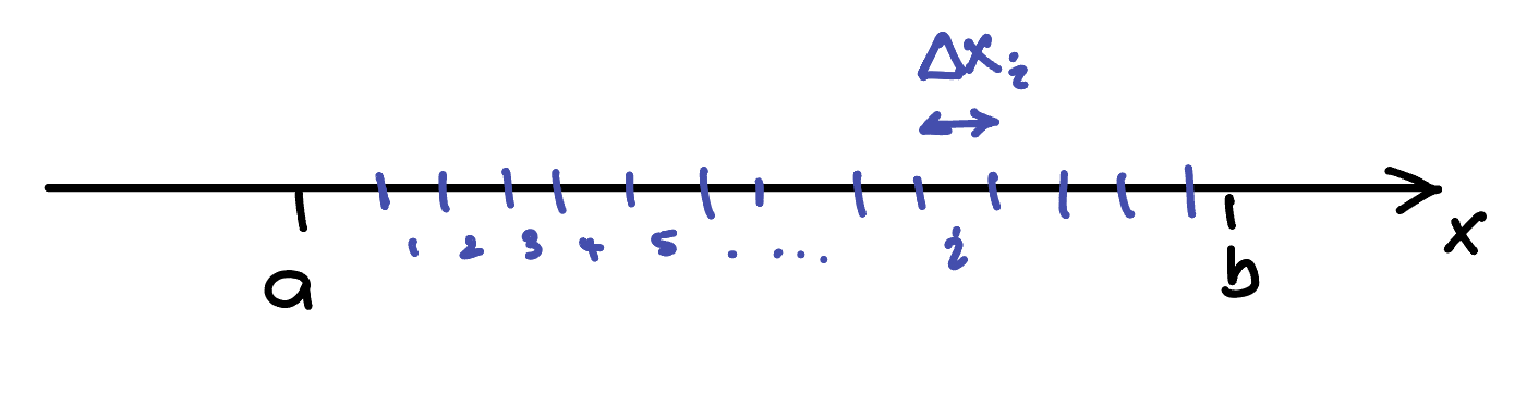
Let us now try to develop a strategy for making sense of what integration actually is. A good place to start is with a fancy-sounding statement called the Riemann Integral/Sum, which you can take as a definition of what integration means:
\[ \int_{x=a}^{x=b} f(x) \, dx \approx \sum_{i=1}^{n} f(x_i^*) \, \Delta x_i \]
Do not panic! This is actually a very cool and simple idea, so let us slowly unpack what it is saying.
- Treat the left-hand side (LHS) as the symbolic or mechanical operation you perform when doing integration.
- The right-hand side (RHS) tells you the meaning of what you are doing; especially the part \(f(x_i^*) \, \Delta x_i\).
- What is happening on the RHS is that we are splitting the interval from \(x = a\) to \(x = b\) into \(n\) small slices, and then calculating the product \(f(x_i^*) \, \Delta x_i\) for each slice. These products represent the area of thin rectangles, and we add them up to get the total.
- The number of slices, \(n\), is up to us. As can be seen in the figure, the more we use, the better the approximation.
- The asterisk in \(x_i^*\) indicates the value of \(x\) we choose within each slice. This, too, is up to us.

(Source: Wikipedia)
Since the approximation improves as \(n\) increases, we can go one step further and imagine the exact area as what we get when we push \(\Delta x\) to zero.
So, integration is really a process of addition, and the meaning of the result depends on the meaning of what you are adding; which is \(f(x) \, \Delta x\).
Examples
Let me try to explain this with a few examples.
\[ \int_{x=a}^{x=b} dx \]
Lets look at the Riemann sum. The figure is a quick sketch of what we are doing. \[ \int_{x=a}^{x=b} dx \approx \sum_{i=1}^{i=n} \Delta x \]
So, the integral, when evaluated will give the legth of a line between \(x=a\) and \(x=b\), which is \(b-a\)
\[ \int_{\theta=\theta_a}^{\theta=\theta_b} r d\theta \]

Lets look at the Riemann sum. \[ \int_{\theta=\theta_a}^{\theta=\theta_b} r d\theta \approx \sum_{i=1}^{i=n} r\Delta \theta \]
Looking at the sketch we see that \(r\Delta \theta\), gives (‘means’) the arc-length of the slice.
So, the integral will give the circumference (or arc length) of the figure.
The expression we get depends on the figure, but the meaning is always the same: we are summing little arcs around the shape.For a circle, where \(r\) is constant: \[ \int_{\theta = \theta_a}^{\theta = \theta_b} r \, d\theta = r(\theta_b - \theta_a) \]
For an ellipse (in polar form), the radius depends on angle \(\theta\): \[ r(\theta) = \frac{a(1 - e^2)}{1 + e \cos \theta} \]
So the arc-length expression becomes: \[ \int_{\theta = \theta_a}^{\theta = \theta_b} r(\theta) \, d\theta \]
This no longer simplifies easily and usually needs to be evaluated numerically.
\[ \int_{\theta=\theta_a}^{\theta=\theta_b} \dfrac{1}{2}r^2 d\theta \]
Compared to the previous example, the only thing we have changed is what is being added. Looking at the sketch, we can see that \(\frac{1}{2} r^2 \, d\theta\) gives (or ‘means’) the area of a small wedge (or sector) of the shape.
So, the integral will give the area of the figure.
As before, the exact expression depends on the shape, but the meaning remains the same: we are summing small areas around the figure.For a circle, where \(r\) is constant: \[ \int_{\theta = \theta_a}^{\theta = \theta_b} \frac{1}{2} r^2 \, d\theta = \frac{1}{2} r^2 (\theta_b - \theta_a) \]
For an ellipse, where the radius depends on the angle \(\theta\): \[ \int_{\theta = \theta_a}^{\theta = \theta_b} \frac{1}{2} r(\theta)^2 \, d\theta \] This typically needs to be evaluated numerically.
Let me now show you two slightly more interesting examples. I won’t go into the Riemann sum here instead, I will point out another neat observation that helps make sense of what’s going on.
\[ \int_{x=a}^{x=b}\int_{y=c}^{y=d} dx\,dy \]
- We are summing little rectangles of size \(\Delta x\,\Delta y\). In other words, we are computing an area.
- From the limits, this is the area of a rectangle: \((b-a)(d-c)\).
\[ \int_{x=a}^{x=b}\int_{y=c}^{y=d}\int_{z=e}^{z=f} dx\,dy\,dz \]
- We are summing little boxes of size \(\Delta x\,\Delta y\,\Delta z\). So we are computing a volume.
- From the limits, this is the volume of a rectangular box: \((b-a)(d-c)(f-e)\).
\[ \int_{r=0}^{r=R}\int_{\theta=0}^{\theta=\pi}\int_{\phi=0}^{\phi=2\pi} r^2 \sin \theta dr\,d\theta\,d\phi \]
- This might seem hard, but it really isn’t. Let’s look at what we are summing:
\[ \begin{align*} &r^2 \sin \theta \, dr\,d\theta\,d\phi \\ =& (\sin \theta)\;\times\; (r\,d\theta)\;\times\; (r\,d\phi)\;\times\; (dr) \\ =& (\text{number}) \;\times\; (\text{length}) \;\times\; (\text{length}) \;\times\; (\text{length}) \end{align*} \]
- So, we are evaluating a volume!
- If you look at the limits, and know what \((r,\theta,\phi)\) represent, you will see that this is the volume of a sphere.
1.3 Partial Derivatives
Motivation
Many interesting systems depend on more than one variable. So it is natural to try to extend our understanding of differentiation to cover such systems.
To help you appreciate how this works, let us start with a simple example: the volume of a cylinder, which is given by:
\[ V = \pi r^2 h \tag{5}\]
Notice how the volume of this system can be changed by either changing the radius \(r\) or the height \(h\).
If we want to study how changing either \(r\) or \(h\) influences the volume of the cylinder, one way to proceed is to keep one variable constant and vary the other. Let’s try that.
If we keep \(r\) constant and change \(h\):
\[ \left.\Delta V \right|_r = \pi r^2 \, \Delta h \tag{6}\]
If we keep \(h\) constant and change \(r\):
\[ \left.\Delta V \right|_h = 2\pi r h \, \Delta r \tag{7}\]
I have obtained the above expressions by purely geometrical reasoning.
The vertical bar ( | ) notation indicates which variable is being held constant.
If you look at these expressions carefully, you will notice that we can rewrite them as follows:
\[ \left.\Delta V \right|_r = \pal{V}{h}{r} \, \Delta h \tag{8}\]
\[ \left.\Delta V \right|_h = \pal{V}{r}{h} \, \Delta r \tag{9}\]
where:
\[ \pal{V}{h}{r} = \pi r^2 \tag{10}\]
\[ \pal{V}{r}{h} = 2\pi r h \tag{11}\]
These ‘curvy’ derivatives are called partial derivatives. You can compute them by treating all variables except the one you’re differentiating with respect to as constants; and then differentiating as usual.
1.4 Uses
Since \(V\) can change in more than one way, we can combine the contributions from \(r\) and \(h\) to write the total differential:
\[ dV = \pal{V}{r}{h} \, dr + \pal{V}{h}{r} \, dh \tag{12}\]
In general, \(dV\), \(dr\), and \(dh\) are called differentials, and you can think of them as conveying the same idea as \(\Delta V\), \(\Delta r\), and \(\Delta h\).
Equation 12 is a very useful statement. For example, we can now study how the volume changes over time based on how \(r\) and \(h\) change over time. All we need to do is write:
\[ \frac{dV}{dt} = \left( \frac{\partial V}{\partial r} \right)_h \frac{dr}{dt} + \left( \frac{\partial V}{\partial h} \right)_r \frac{dh}{dt} \tag{13}\]
This tells us how the volume evolves in time by accounting for the individual rates at which the radius and height change.
Take a look at the nice example that Ryan has written for you to illustrate this.
One of the other important uses of partial derivatives is in understanding how measurement errors or uncertainties in one variable can lead to (or propagate) into errors in other variables. We will explore this important idea further in a later section.
2 Probability Distributions
2.1 What Is a Probability Distribution?
In this chapter, I want to introduce tools that help us understand and talk about the systems we study. Calculus gave us a way to describe change, and to build models that help us understand the dynamics of a system how it evolves in time or space. But there is another kind of knowledge that is just as important, and often more practical when we deal with the real world.
I am referring to a statistical understanding of a system that allows us to connect our mathematical models to actual measurements and experimental results. This is where probability distributions become essential.
To illustrate the difference: Newton’s laws (expressed as differential equations) can help us predict how two balls will collide and move apart. But if I were to repeat this experiment 1000 times, the balls would scatter differently each time. While each individual collision still follows Newton’s laws, those laws alone are not enough to answer questions like, ‘how many balls will scatter at an angle of 90 degrees?’
To answer that kind of question, we need a statistical interpretation. We need a way to describe how likely different outcomes are; Even if we cannot predict each one individually. This is exactly what a probability distribution provides: a framework for answering questions about patterns, frequencies, and expectations across many events or measurements.
2.2 Types of Probability Distributions
Probability distributions come in two main flavours: discrete and continuous.
(Source: Medium)

(Source: Wikipedia)
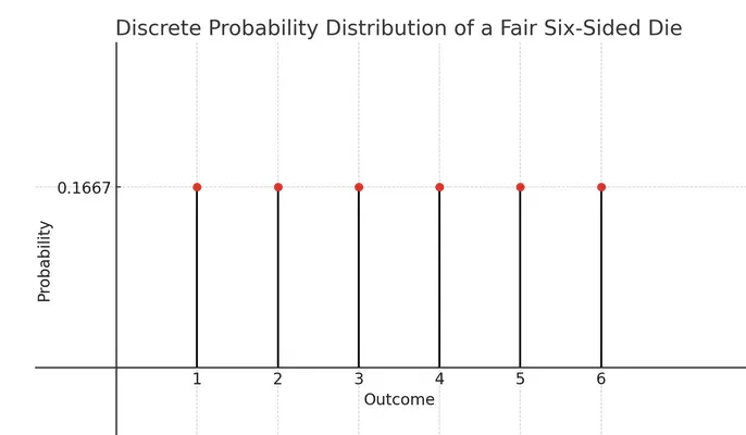
Discrete Distributions
- A discrete distribution tells us the probability of observing specific, separate outcomes.
A simple example is the probability distribution for a fair six-sided die, shown in Figure 5. - Only distinct, countable values are shown. Each outcome has a well-defined probability.
- Discrete distributions are represented by a Probability Mass Function (PMF), usually written as \(f(i)\) or \(P(i)\), where \(P(i)\) gives the probability of the value \(i\) occurring.
- The total probability over all possible outcomes must add up to 1:
\[ \sum_i f(i) = 1 \]
Continuous Distributions
- Continuous distributions describe the probability of outcomes lying within a continuous range of values.
An example is the uniform continuous distribution between \(a\) and \(b\), shown in Figure 6. - For continuous variables, the probability of a single value is zero. Instead, we talk about the probability of a value falling within an interval, which is computed using an integral.
- Continuous distributions are represented by a Probability Density Function (PDF), written as \(f(x)\).
- The function \(f(x)\) itself is not a probability. Instead \(f(x) \, dx\) is the probability of \(x\) falling within a small interval \([x, x + dx]\).
- The probability of \(x\) falling within a finite interval \([a, b]\) is:
\[ \int_a^b f(x) \, dx \] - The total probability across the entire domain must equal 1:
\[ \int_{-\infty}^{\infty} f(x) \, dx = 1 \]
3 Error Analysis & Error Propagation
When we repeat the same measurement many times, we almost never get exactly the same value each time. Instead, the results vary and spread out. This makes it difficult to decide on a single ‘true’ value. We use the terms error or uncertainty to describe this spread in results.
This variability can arise from many sources; some due to the measurement process itself, and others due to the nature of the system. In fact, some systems (like those in quantum mechanics) have an inherent probabilistic behaviour, which naturally leads to a distribution of outcomes. The science (and art) of error analysis is about carefully examining our experiments and data to quantify how much confidence we can place in our results.
Another facet of error analysis is error propagation. Experiments are rarely straightforward and it is common to measure several different quantities in order to infer a final result that we are truly interested in. In such cases, an important aspect of error analysis is error propagation, which allows us to understand how uncertainties in the measured quantities influence the uncertainty in the final result.
To make sense of this topic, we will need a few key statistical ideas and formulas.
3.1 Useful Ideas from Stats
Parent vs Sample Populations
If we could measure a system infinitely many times, we would know all possible outcomes. This complete distribution is called the parent distribution. In reality, we only make a finite number of measurements. These form a sample, which is our best approximation to the parent distribution.
\[ \text{Parent distribution} = \lim_{N \to \infty} \; \text{Sample distribution} \tag{14}\]
The whole point of error analysis is to use our sample population to infer the detials of the parent.
Mean
If \(x_1, x_2, x_3, \dots, x_N\) are independent measurements, the mean (or average) is defined as:
\[ \bar{x} = \frac{1}{N} \sum_{i=1}^{N} x_i \tag{15}\]
We usually take the mean to be the most representative value from a set of measurements. This relies on the idea that the errors in the measurement process are random so that with enough measurements, the positive and negative deviations tend to cancel out. The larger the number of measurements, the more effective this cancellation becomes.
Standard Deviation
The standard deviation, denoted by \(s_x\), gives us an idea of how spread out the measurements are around the mean \(\bar{x}\). It is defined using the following biased estimate2:
\[ s_x^2 = \frac{1}{N-1} \sum_{i=1}^{N} (x_i - \bar{x})^2 \tag{16}\]
This form with \(N - 1\) in the denominator gives the best estimate of the standard deviation of the parent population based on a finite sample. That said, the difference between \(N\) and \(N - 1\) becomes negligible quite quickly as \(N\) increases. In practice, this distinction only matters for small sample sizes. As a general rule, we should aim to make \(N\) as large as possible.
How large is “large enough” depends on the experiment and the desired level of precision. Typically, an experiment is repeated multiple times, with incremental refinements, until the results reach the level of accuracy or confidence required.
Two Important Laws
Best Estimate
Based on the ideas above, the best estimate of a measured quantity and what you should report is:
where:
- \(\bar{x}\) is the sample mean (see Equation 15),
- \(s_x\) is the sample standard deviation (see Equation 16),
- \(N\) is the number of measurements you used to determine these.
The term \(\dfrac{s_x}{\sqrt{N}}\) is called the standard error. It gives us our best estimate of the confidence we can place in the reported mean. I will shortly prove how this standard error arises.
Propagation of Errors
Let me take a specific example — the volume of a cylinder, given by
\(V = \pi r^2 h\) — to introduce the idea of Propagation of Errors.
A natural place to start is with the total derivative of Equation 12:
\[ dV = \pal{V}{r}{h} \, dr + \pal{V}{h}{r} \, dh \]
Let me now rewrite this in a more suggestive (but approximate) form:
\[\begin{align} \Delta V &\approx \pal{V}{r}{h} \, \Delta r + \pal{V}{h}{r} \, \Delta h \\ &\approx (2\pi r h) \, \Delta r + (\pi r^2) \, \Delta h \end{align}\]
Now, dividing everything by \(V = \pi r^2 h\), we get:
\[ \f{\Delta V}{V} \approx 2\lr{\f{\Delta r}{r}} + \lr{\f{\Delta h}{h}} \tag{19}\]
Equation 19 gives us the fractional (or percentage) error in \(V\) based on the percentage errors in \(r\) and \(h\).
Notice something important: the error in \(r\) contributes twice as much as the error in \(h\). This tells us that we need to measure \(r\) more carefully if we want to keep the error in \(V\) small.
So, partial derivatives are incredibly helpful — they tell us which parts of an experiment contribute most to the uncertainty in the final result.
However, Equation 19 is not the best way to estimate the final uncertainty in \(V\). Why?
Because it assumes the worst-case scenario — that both \(r\) and \(h\) reach their maximum possible errors at the same time, and in the same direction. This is very unlikely in real experiments where errors are random. So, while this expression is useful for understanding, it tends to overestimate the total error and can be too conservative.
We need a more refined way to combine errors — one that takes the random nature of measurement uncertainties into account.
The Error Propagation Formula
It turns out (see Bevington and Robinson 2003, chap. 3; also Taylor 1997, chap. 5) that the best way to combine uncertainties is by using the Error Propagation Formula.
This is a very general and powerful result. It tells us how to propagate uncertainties from independent input variables into a derived quantity. The key assumptions are that the variables are independent and that their uncertainties are random and uncorrelated. The formula is flexible and can be applied to a wide range of functions: products, powers, logarithms, exponentials, and trigonometric expressions.
4 A Useful Approximation
4.1 Taylor Series
I would like to wrap up this chapter by introducing you to a simple idea that will help you in many different situations. It is called the Taylor series expansion, and it allows you to think of a function as a series of powers.
More formally, the Taylor series of a function \(f(x)\) around a point \(x = x_0\) is defined as:
\[ f(x) = f(x_0) + f'(x_0)(x - x_0) + \frac{f''(x_0)}{2!}(x - x_0)^2 + \frac{f^{(3)}(x_0)}{3!}(x - x_0)^3 + \cdots \]
It is important to keep in mind that this is an approximation that is built around a specific point: \(x = x_0\). The farther you move away from this point, the less accurate the approximation becomes. How far is “too far” depends on the function you are working with.
4.2 Maclaurin Series
Here are the Taylor series for some commonly used functions around \(x = 0\). This special case where the expansion is about zero is called the Maclaurin series.
\[ e^x = 1 + x + \frac{x^2}{2!} + \frac{x^3}{3!} + \cdots \tag{21}\]
\[ \sin x = x - \frac{x^3}{3!} + \frac{x^5}{5!} - \frac{x^7}{7!} + \cdots \tag{22}\]
\[ \cos x = 1 - \frac{x^2}{2!} + \frac{x^4}{4!} - \frac{x^6}{6!} + \cdots \tag{23}\]
\[ \tan x = x + \frac{x^3}{3} + \frac{2x^5}{15} + \frac{17x^7}{315} + \cdots \tag{24}\]