Ideas for Telling Stories

Taking a Fresh Look at Some Old Ideas

Figure 1: The ability to explain and understand concepts in simple terms is both valuable and important.

He who knows nothing, loves nothing. He who can do nothing understands nothing. He who understands nothing is worthless. But he who understands also loves, notices, sees… The more knowledge is inherent in a thing, the greater the love. Anyone who imagines that all fruits ripen at the same time as the strawberries knows nothing about grapes.
– Paracelsus

Words of wisdom, the meaning of life, perhaps even the answer sought by Borges’s librarians — all of these may wash over us every day, but they can do little for us unless we savor them,engage with them, question them, improve them, and connect them to our lives.
– Jonathan Haidt

The greatest enemy of knowledge is not ignorance, it is the illusion of knowledge
– Daniel J. Boorstin

What To Expect In This Chapter

This chapter is devoted to the fundamental concepts and ideas. We will introduce some new ones and strengthen the ones you already know. These ideas will become the building blocks that help you tell stories about science.

Part of the difficulty in understanding physics comes from the fact that many technical terms (like ‘force’, ‘energy’, or ‘work’) are also used in everyday life, but with looser meanings. More subtly, we often go around with the illusion that these are simple ideas we already know well. Here, we will sharpen those meanings and connect them to one another. My hope is that you will develop a clear picture of the meaning and interconnections between concepts such as force and energy, and energy and temperature. Try to look at these ideas from multiple perspectives and put your understanding to the Aunty Test.

Finally, recognise that there is always a story behind every concept and equation. An equation is more than a formula: it captures an intuitive idea about how the world works. Appreciate how mathematics can not only express these intuitions with elegance, but also empower us to go further and develop insights and make predictions.

1 Vectors & Scalars

We can categorise physical quantities (such as temperature, force, energy, or distance) as either scalars or vectors.

Scalar A scalar can be fully described by just a number (its size or magnitude). Examples include mass (50 kg), temperature ($-20\,^\circ$C), distance (100 km), and height (180 cm). Scalars are often easier to work with because they are simply numbers.

Vector A vector, on the other hand, requires two pieces of information: a magnitude (a number) and a direction. Examples include force (10 N downwards), velocity (50 km/h due north), and displacement (10 m to the left).

We usually represent a vector with an arrow: the arrow’s length shows the magnitude, and its orientation shows the direction. In writing, we often add a small arrow above the symbol ($\vec{X}$) or make it bold ($\mathbf{X}$). The magnitude of a vector is written without the arrow, either as $X$, $|\vec{X}|$, or $|\mathbf{X}|$.

Figure 2: A vector has a size and a direction.

1.1 Components & Resultant Of A Vector

Adding and subtracting vectors is interesting because we must take direction into account. Two key ideas here are the resultant and components.

Resultant As shown in Figure 4, two vectors can be combined (added) to give a single vector. This is called the resultant, and it has the same overall effect as the original vectors combined. The standard way to add vectors is to draw them end to end.

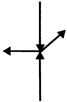
Components Just as we can combine vectors to form one, we can also reverse the process and split a vector into parts, called its components. Figure 3 shows three ways of splitting one vector ($\vec{F}$, shown in colour) into two others¹. The most common and useful choice is to split into two perpendicular directions (leftmost).

Figure 3: Three ways the same vector (shown in **colour**) is split into components.

Figure 4: Two or more vectors can be added to give a single resultant vector. In this example the resultant $\vec{R}$ produces the same effect as the combination of vectors $\vec{F}_1$ and $\vec{F}_2$.

Perpendicular components

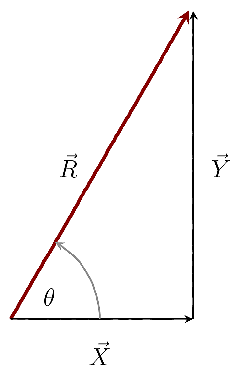
One convenient way to split a vector is into two (or three, in 3D) perpendicular components. In such a situation we can obtain the resultant vector using Pythagoras’ theorem. For the situation shown in Figure 5, the size and direction of the resultant are:

\[ |\vec{R}| = R = \sqrt{X^2 + Y^2} \tag{1}\]

\[ \tan \theta = \dfrac{Y}{X} \tag{2}\]

If you have three perpendicular components $\vec{X}, \vec{Y}, \vec{Z}$ then:

\[ |\vec{R}| = R = \sqrt{X^2 + Y^2 + Z^2} \tag{3}\]

Figure 5: Resultant of two perpendicular vectors.

1.2 Play with vectors

You can try out the ideas above using the following applet (from PhET Interactive Simulations (2025)).
For instance Use the applet (Lab) to find the resultant of the set of vectors shown in the adjoining figure.

2 Speed, Velocity and Acceleration

Speed (ms^-1) tells us how fast something is moving relative to a point of origin.
Velocity (ms^-1) tells us how fast and in which direction it is moving.
Acceleration (ms^-2) tells us how fast the velocity is changing.

Mathematically:

\[ v=\da{x}{t} \tag{4}\]

\[ \vec{v}=\da{\vec{x}}{t} \tag{5}\]

\[ \vec{a}=\da{\vec{a}}{t} \tag{6}\]

3 Forces

3.1 What is a force?

A force is simply a push or a pull.

A force is a vector, so we need to specify both direction and magnitude to describe it completely. As shown in Figure 7, when a (net) force acts on a mass it changes the velocity of the mass. I.e. a force can change the speed and the direction of motion. The SI unit of force is the Newton (N)².

Figure 7: A force can change the velocity of a mass.

3.2 Newton’s Laws

From everyday experience we know that more force means more acceleration³, and more mass means less acceleration. We capture this mathematically as

\[ a = \dfrac{F}{m} \tag{7}\]

This is Newton’s Second Law, which helps us quantify the effect of a force.

Newton’s First Law tells us what a force does. It states that an object will continue in its state of rest or uniform (unaccelerated) motion in a straight line unless acted upon by an external (resultant) force.

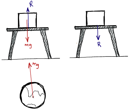
Newton’s Third Law is about how forces occur. It states that when an object A exerts a force on object B, object B exerts an equal and opposite force on object A. You can see this in Figure 8 where I have draw the the various action-reaction pairs.

Figure 8: Forces always occur in pairs and always involves two bodies.

Example 1 (Constant force on an object)

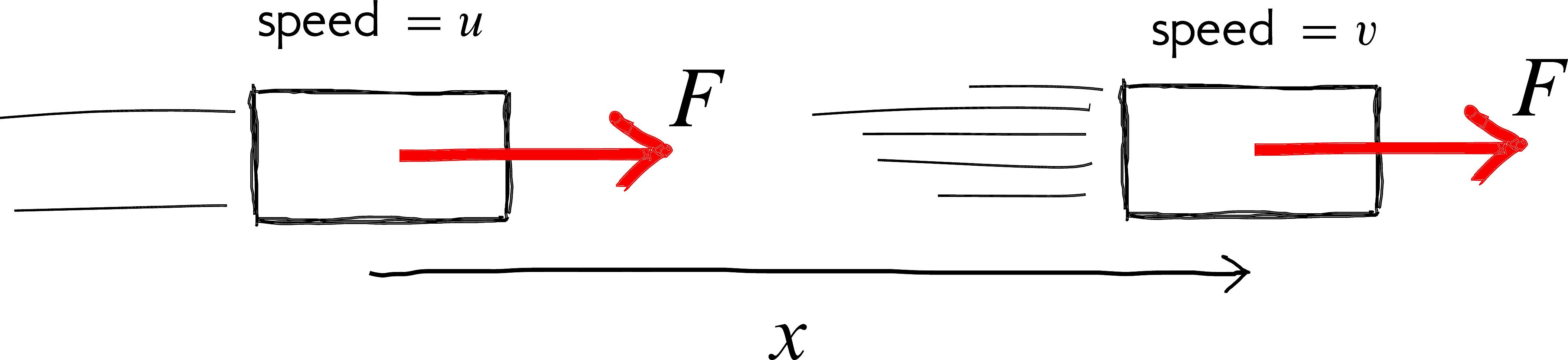
Figure 9: A constant force $F$ acting on a mass over a distance $x$.

Consider the situation in Figure 9 where a constant force acts on a mass over a distance $x$.

Starting with Newton’s Second Law and using the chain rule,

\[ \begin{aligned} F &= m a = m \frac{dv}{dt} = m \frac{dv}{dx}\,\frac{dx}{dt} = m v \frac{dv}{dx} \\\\ \Rightarrow \frac{F}{m} &= v \frac{dv}{dx} \\\\ \frac{F}{m} \int_{0}^{x}\!dx &= \int_{u}^{v}\!v\,dv \\\\ a\,[x]_0^x &= \left[\frac{1}{2}v^2\right]_u^v \quad \text{(for constant $a$)} \\\\ \therefore \; a x &= \frac{v^2-u^2}{2} \end{aligned} \]

which leads to

\[ v^{2}=u^{2}+2ax \tag{8}\]

This equation matches intuition: the final speed increases with the distance over which the force acts; if there is no force ($a=0$), the speed remains steady.

Example 2 (More Stories)

While we are here, let me tell you a story using Equation 8.

Imagine you are driving at a speed $v_{start}$ and you apply the brakes to come to a stop. What will your stopping distance be?

With $u = v_{start}$ and $v = 0$, we get

\[ x_{stopping} = -\frac{v_{start}^2}{2a} \]

Here $a$ must be negative, since the car is decelerating. Suppose you press the brakes as hard as possible, giving the maximum deceleration the car can manage. Then the stopping distance becomes

\[ x_{stopping} = \frac{v_{start}^2}{2a_{max}} \]

This is a slightly scary result! It tells us that if you double your speed (say, from 30 to 60 km/h), your stopping distance will quadruple. That is why overtaking can be risky if not done carefully: you are going faster than the car you are passing, and if you suddenly have to stop, you will almost certainly run into it.

4 Mass, Inertia & Momentum

4.1 Mass & Inertia

Mass tells us how much matter an object contains and is a fundamental property⁴. Mass is also a measure of how resistant the object is to changes in its motion. This resistance is what we call its inertia.

Because of inertia, an object at rest tends (‘likes’) to remain at rest, and an object in motion tends (‘likes’) to keep moving in a straight line⁵. This idea is captured in Newton’s First Law.

4.2 Momentum?

What is Momentum?

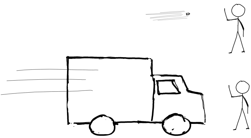
As Figure 10 tries to highlight, everyday experience tells us that the ‘hurt’ from an impact depends on the combination of mass ($m$) and speed ($v$). It is common to see this combination of mass and speed throughout science. More correctly, this quantity is a vector called momentum, defined as

\[ \vec{p} = m\vec{v} \tag{9}\]

Its unit is $\mathrm{kg\,m/s}$. Momentum has deep connections across physics: it appears in the definition of force, plays a central role in quantum mechanics, and is one of the fundamental quantities conserved in our Universe.

Momentum is conserved

Some quantities in our Universe (such as energy) are conserved, meaning they remain unchanged under certain conditions. These conservation laws are usually linked to deeper structures called symmetries (for example, translational symmetry) of our Universe⁶.

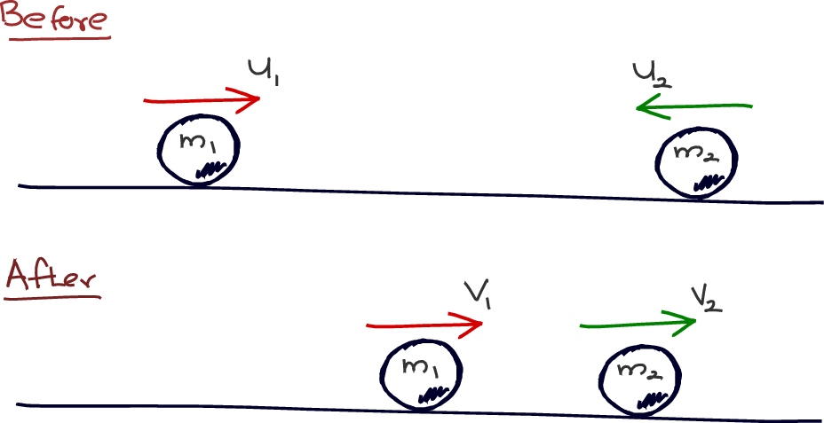
Momentum is one of the conserved quantity. So, the total momentum of a system stays constant as long as no external forces act on it. For the system shown in Figure 11,

\[ m_{1} \vec{u}_{1} + m_{2}\vec{u}_{2} = m_{1}\vec{v}_{1} + m_{2}\vec{v}_{2} \tag{10}\]

Figure 10: A fast light bullet can hurt you as much as a slow massive lorry.

Figure 11: Momentum is conserved. The total momentum before and after is the same if there are no external forces.

Momentum & force

A force is really about how fast momentum is changing. In fact, Newton defined force as the rate of change of momentum:

\[ F = m a = m\dfrac{dv}{dt}= \dfrac{d(mv)}{dt}= \dfrac{dp}{dt} \tag{11}\]

Example 3 ($\Delta \vec{p}$ for a bouncing ball)

We can now use what we know to analyse interesting situations.
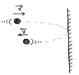
For instance, what is the force exerted on a ball of mass $m$ that hits a wall and reverses direction with the same speed $v$?

\[ \Delta \vec{p} = \vec{p}_{\text{after}}-\vec{p}_{\text{before}} = m\vec{v} - m(-\vec{v}) = 2m\vec{v}. \]

If the time of contact is $\Delta t$, then from Equation 11, \[ F = \dfrac{\Delta \vec{p}}{\Delta t}. \tag{12}\]

Figure 12: What is the change in momentum when a ball bounces off a hard wall?

If you are wondering why this is interesting, think about what it means for the wall: it experiences the same force in the opposite direction! In fact, this idea is the starting point of the kinetic theory, which explains how a gas exerts pressure.

4.3 Energy

Energy is such a central concept in our understanding of the Universe that it is important to make sense of what it really is. Let us begin with a simple, intuitive description of energy.

Energy is the ability to do ‘something useful’.

As seen Figure 13, ‘useful’ is not well-defined. So, this definition is imprecise; we will refine it once we define work.
The S.I. unit of energy is the Joule (J). Energy is also a conserved quantity⁷.
There are many forms of energy (e.g. light, heat, potential energy, kinetic energy). Here are two forms of energy that we encounter often:

Kinetic Energy \[ \text{KE} = \f{1}{2}mv^2 \]

Potential Energy \[ \begin{align} \text{Gravitational PE} &= mgh\\ \text{Elastic PE} &= \f{1}{2}kx^2\\ \end{align} \]

Figure 13: The potential energy of the block being converted to do something useful.

4.4 Work

Forces can transfer energy

If you recall an instant when you used a force, you will realise that forces also do another very important thing.

A force allows us to transfer energy.

Whenever you lift or push an object, you transfer energy from one form to another (e.g. lifting: chemical to $PE$; pushing: chemical to $KE$) through the action of a force. A force does not always facilitate the transfer of energy (e.g. when you are pushing a wall).

This idea of forces transferring energy is essential to understand how energy makes our Universe work. We use the concept called work to quantify the ‘energy transferring ability’ of a force.

The Definition of Work

Figure 14: A constant force acting on an object.

Figure 15: A variable force acting on an object.

The amount of energy transferred by a force is called the work ($W$) done by the force and is given by:

Definition of Work

\[ W=\begin{cases} F\,x \cos \theta & \text{(constant force)}\\\\ \displaystyle \int F\,\cos \theta \, dx & \text{(variable force)} \end{cases} \tag{13}\]

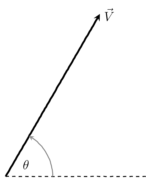
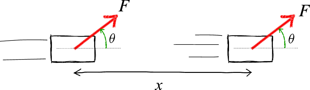
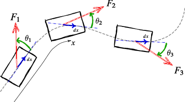
Here, $\theta$ is the angle between the force and the direction of motion (the direction of $\vec{x}$ or $dx$), as shown in Figure 14. The integral form in Equation 13 is the most general because it handles situations where things change (e.g. the angle), as in Figure 15.

It is important to note that energy is a scalar quantity: it is described only by a number. However, this number can be positive or negative. The sign tells us whether work is adding to the energy of an object or taking energy away from it. Let’s look at some examples to help understand the idea of work.

Example 4 (Work & Kinetic Energy)

Figure 16: A constant force acting on an object.

To demonstrate the power of the definition of work, let us use it to derive the expression for kinetic energy ($KE$), for the case shown in Figure 16.

The work done by a constant force $F$ over a distance $x$ is

\[ W = F x \cos 0^\circ = m a \, x \]

Using Equation 8:

\[ W = m \left(\frac{v^{2}-u^{2}}{2x}\right) x \]

\[ W= \frac{1}{2}mv^{2}-\frac{1}{2}mu^{2}. \]

Thus the energy transferred by the force appears as a change in the quantity $\dfrac{1}{2}mv^2$, which we identify as a measure of the kinetic energy of the object.

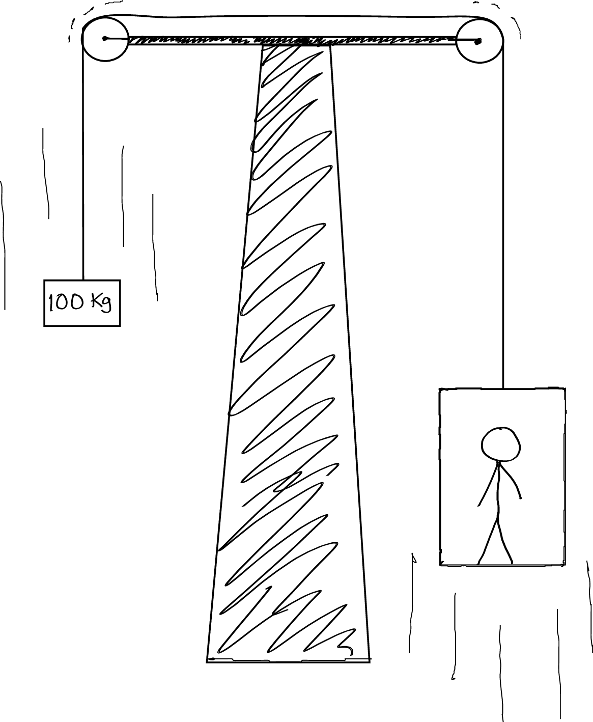
Example 5 (Who does work?)

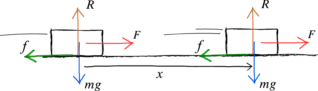
Figure 17: Let us determine the work done by all the forces acting on the object.

Consider the situation in Figure 17. A constant force ($F$) acts on a mass that also experiences friction ($f$), weight ($mg$)⁸ and a normal reaction from the ground ($R$). The table below shows the work done by each of the forces.

Work done by each force (over a horizontal displacement $x$):

Force	Angle ($^\circ$)	Work
Push ($F$)	$0$	$Fx\cos 0 = Fx$
Contact force ($R$)	$90$	$R x \cos 90 = 0$
Weight ($mg$)	$90$	$mg\, x \cos 90 = 0$
Friction ($f$)	$180$	$f x \cos 180 = -fx$
Total work		$(F-f)x$

Table 1: Work done by the various forces acting on the object.

Note that not all forces do work. The positive work transfers energy into increasing the object’s $KE$; negative work (e.g. friction $f$) removes $KE$. We often say that $F$ does work against $f$.

The total energy transferred and the $KE$ gained is

\[ \text{Total work done} = (F-f)x = \Delta(\mathrm{KE}). \tag{14}\]

4.5 Definition of Energy

Now that we understand what work is, we can sharpen our definition of energy:

Energy is the ability to do work.

Boltzmann’s Distribution Law & Temperature

5 What is Temperature?

The sense of hot and cold (temperature) is a manifestation of the constant motion (kinetic energy) of the particles that make up matter. The more energy we give particles, the faster they move, and the higher the temperature. The average kinetic energy of a population of particles is related to its temperature as

\[ \overline{\mathrm{KE}} \propto k_B T \tag{15}\]

where $k_B = 1.381 \times 10^{-23}\,\mathrm{J\,K^{-1}}$ is Boltzmann’s constant.

Notice that the concept of temperature only makes sense for a large number of particles. The quantity $k_B T$ represents the typical thermal energy scale at temperature $T$, and it plays a central role across the physical, chemical, and biological sciences.

5.1 Boltzmann’s Distribution Law

Temperature has a deeper meaning than just being related to kinetic energy. A better way to understand temperature is as a measure of how particles are distributed among different energies under the constant jostling and bustling of motion.

This idea is captured by Boltzmann’s Distribution Law, which can be regarded as the true meaning of temperature.
It has an astonishingly simple form:

\[ \frac{N_j}{N_i} = e^{-\f{E_j - E_i}{k_B T}} = e^{-\f{\Delta E}{k_B T}} \tag{16}\]

where $N_i$ and $N_j$ are the numbers of particles in energy states $E_i$ and $E_j$, respectively.

The Boltzmann distribution applies to any (classical⁹) system with different possible energy states. You can think of it as the kinetic energy ‘shuffling’ particles between available states until the system settles into a dynamic equilibrium: particles continuously move in and out of energy states, but the overall distribution remains steady. We describe this steady distribution as having a constant temperature $T$.

The Boltzmann distribution is everywhere! It governs chemical reactions, how proteins fold, how quantum systems fluoresce, and much more. Sometimes, understanding a system becomes almost trivial once you recognise that it is, at its heart, a Boltzmannian system.

Example 6 (A Gas In A Cylinder) Let me now work a simple example that brings together many of the ideas we have discussed in this chapter so far.

Consider a gas contained in a cylinder of cross-sectional area $A$, maintained at a temperature $T$.

We begin with the ideal gas law: \[ pV = NRT \]

where $N$ is the number of moles of gas.

Since, $R \equiv N_A k_B$ the pressure can be expressed as \[ p = \frac{N N_A}{V} k_B T \Rightarrow \boxed{p= n k_B T} \] where $n$ is the number density (particles per unit volume).

Now, lets consider a thin slab of thickness $dh$ and area $A$ at height $h$.

Since, the gas is in equilibrium:

\[ (\text{Forces down}) = (\text{Forces up}) \]

\[ Mg + (p + dp)A = pA, \]

where $M$ is the mass of the slab and is given by \[ M = \big[n(A \, dh)\big] m. \]

where, $m$ is the mass of a single particle.

Thus, \[ A \, dp = - Mg = - n m g A \, dh \]

\[ \Rightarrow \boxed{dp = - n m g \, dh} \]

Looking at the top, boxed equation, \[ p = n k_B T \Rightarrow dp = dn \, k_B T. \]

Therefore, \[ k_B T \, dn = - n m g \, dh. \]

Separation of variables \[ \frac{dn}{n} = - \frac{mg}{k_B T} \, dh. \]

Integrating, \[ \int_{n_0}^n \frac{dn}{n} = - \int_0^h \frac{mg}{k_B T} \, dh. \]

\[ \ln \frac{n}{n_0} = - \frac{mgh}{k_B T}. \]

Leaving us with: \[ n = n_0 e^{-\dfrac{mgh}{k_B T}}. \]

or equivalently, \[ \frac{n}{n_0} = e^{-\dfrac{\Delta E}{k_B T}}. \]

This is exactly the Boltzmann Distribution Law! It tells us about the equilibrium reached when the kinetic energy of the particles (represented by $k_B T$) continually shuffles them among energy states, sometimes kicking them upwards.

If we had recognised this earlier, we could have simply written down the law!

5.2 Maxwell–Boltzmann Distribution of Speeds

You are probably more familiar with the Maxwell–Boltzmann distribution of particle speeds than with the (original) Boltzmann distribution . Let’s focus on the Maxwell–Boltzmann distribution, because it is extremely useful for understanding many systems where temperature plays a key role. It also gives us a nice opportunity to see how the characteristics of a specific system (e.g. it dimensionality) modify the underlying Boltzmann distribution.

The (original) Boltzmann distribution is a very general statistical law. It tells us the probability that a system occupies a state of energy $E$ at temperature $T$:
\[ P(E) \propto e^{-E/k_B T}. \]
In other words, it describes how energy is distributed among possible microscopic states.

The Maxwell–Boltzmann distribution is a special application of the Boltzmann distribution to the motion of gas particles. Instead of energy levels in general, we now ask: what is the probability that a particle has a certain speed $v$? This requires taking the Boltzmann factor $e^{-E/k_BT}$, with $E = \f{1}{2} m v^2$, and combining it with the number of velocity states available at that speed. The result is the familiar distribution of particle speeds. This distinction is important: here we are looking at speeds, the magnitude of velocity.

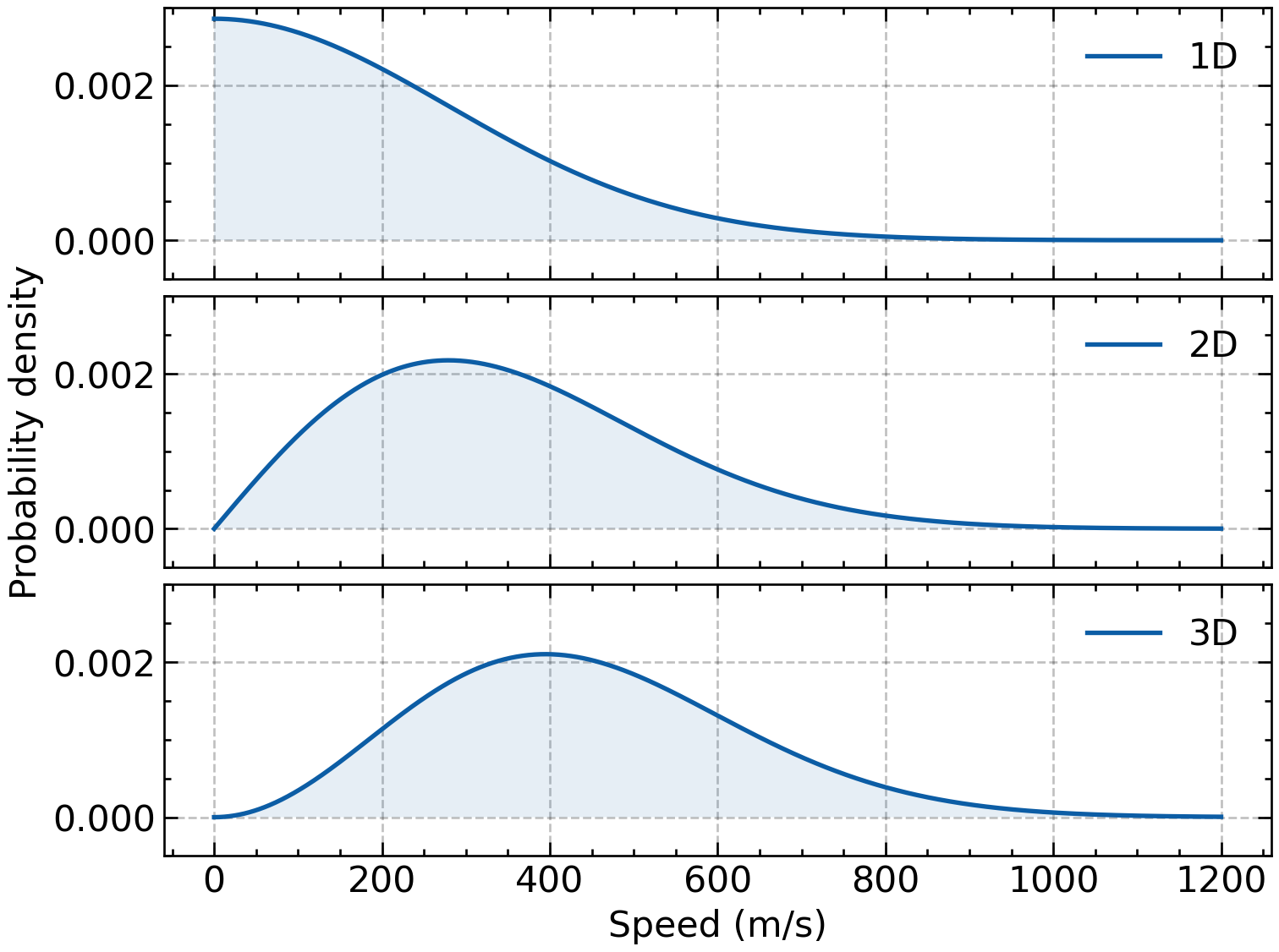
For a system at temperature $T$, particle mass $m$, and Boltzmann constant $k_B$, the Maxwell–Boltzmann distribution of speeds depends on the number of spatial dimensions $D$.

\[ \begin{align} \text{Speed Distribution in 1D: }\qquad f(v_x) &= \sqrt{\f{2}{\pi}}\lr{\f{m}{k_B T}}^\frac{1}{2} \,v^0\, e^\left(-\f{\frac{1}{2}m v_x^2}{k_BT}\right) \\[1em] \text{Speed Distribution in 2D: }\qquad f(v) &= \lr{\f{m}{k_B T}} \, v^1 \, e^\left(-\f{\frac{1}{2}m v^2}{k_BT}\right) \\[1em] \text{Speed Distribution in 3D: }\qquad f(v) &= \sqrt{\f{2}{\pi}}\lr{\f{m}{k_B T}}^\frac{3}{2} v^2 e^\left(-\f{\frac{1}{2}m v^2}{k_BT}\right) \end{align} \]

Figure 18: 1D, 2D and 3D Maxwell-Boltzmann Distributions for T=300 K.

These different distributions arise because of the number of ways a given speed can be realised in different dimensions.

In 1D, the speed is just one number: $v_x$.
In 2D, a single speed can come from many different velocity pairs $(v_x, v_y)$ that satisfy $v = \sqrt{v_x^2 + v_y^2}$.
In 3D, there are even more combinations of $(v_x, v_y, v_z)$ that give the same speed $v = \sqrt{v_x^2 + v_y^2 + v_z^2}$.

So, as the dimensionality increases, the number of ways to achieve a particular speed increases, and this shows up as the extra factors of $v$ or $v^2$ in the 2D and 3D Maxwell–Boltzmann speed distributions.

What I would like you to notice is that the specific characteristics of the system we are considering influences how the Boltzmann energy distribution describes it. For example:

In a gas, the relevant energy is the kinetic energy of particles, and the Boltzmann distribution leads us directly to the Maxwell–Boltzmann speed distributions.
In a system of molecules with quantised energy levels (e.g. vibrations or rotations), the same Boltzmann factor explains why lower energy states are more populated, yet higher states still have some probability.
In biological systems, like DNA folding, the ways that DNA can fold will influence how they are distributed..

So the Boltzmann distribution is the foundation, but the way it looks in practice depends on the nature of the system.

Shown below are the Maxwell–Boltzmann speed distributions for three different temperatures. Notice how the shape changes:

At low $T$, the distribution is narrow and peaked at lower speeds.
At higher $T$, the peak shifts to the right (higher most-probable speed) and the curve broadens.
At very high $T$, the distribution flattens further — more particles occupy higher speed states.

Figure 19: Three Temperature for Maxwell Boltzmann Distribution in 3D.

6 Interaction Cross Sections

6.1 The Idea of a Cross-Section

Now I like to introduce a concept that you might not encounter elsewhere, but which is very useful when thinking about how interactions occur. It also provides us with a practical way to design experiments and analyse results even if we don’t yet completely understand all of the underlying science.

This concept is called a cross-section.

6.2 A Simple Model For A Cross-Section

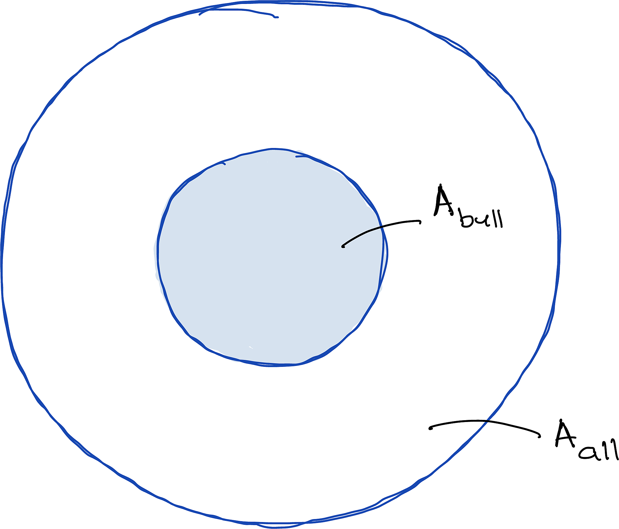
It is simpler to understand the concept of a cross-section in the context of many particles impinging on a target. Let’s start simply with the adjoining figure. It is reasonable to assume that if we throw a large number of darts (say $N_0$), then the number of darts that hit the bull’s eye (say $N_\text{bull}$) satisfies:

\[ \def\ax{\text{area}_\text{bull}} \def\bx{\text{area}_\text{all}} \f{N_\text{bull}}{N_0}=\f{\ax}{\bx} \tag{17}\]

Notice how $\ax$ gives us a sense of how often a dart will interact with the bullseye. We use the term cross-section to describe this ‘sense’. The bigger the area of the bull’s eye, the bigger the cross-section, and the greater the chance of a ‘hit’.

6.3 Total Cross-Section: A Happy Way

I will now use a frivolous, ‘happy’ model to further develop the ideas of cross-sections. But don’t worry, I will make it more serious later.

Single Centre

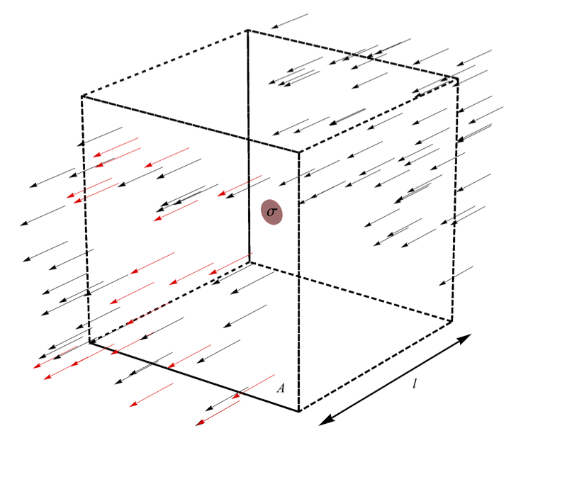
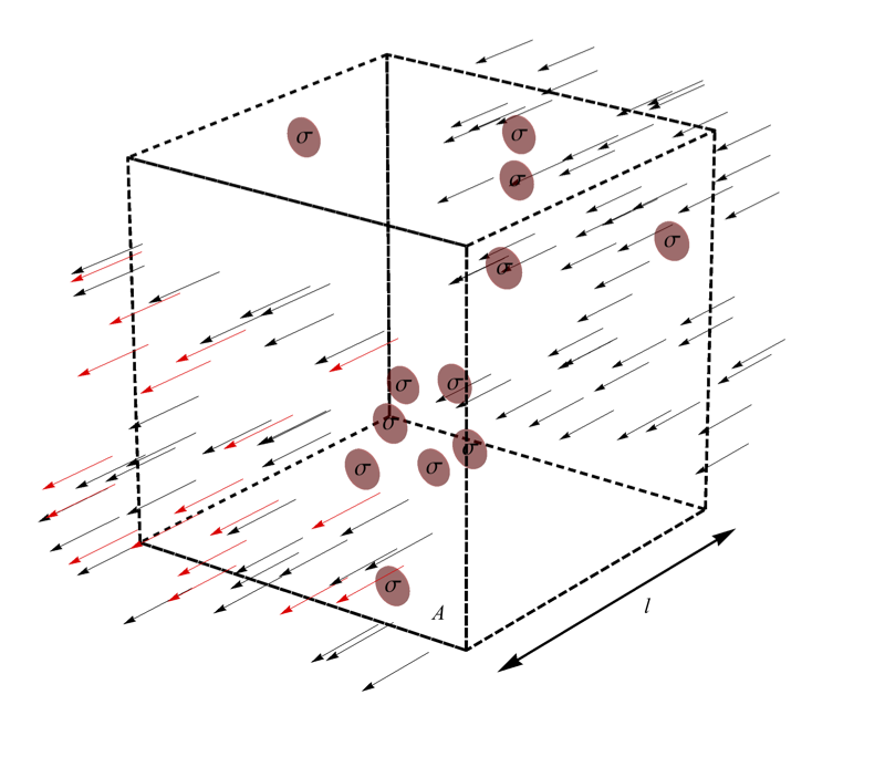
The adjoining image shows projectiles passing through a sample of area $A$ and thickness $l$. During the journey, some projectiles interact with the ‘happiness’ centre (shown in colour). When the particles interact, they become ‘happier’. Let’s denote happiness with $H$ and allow it to take a value between 0 and 1 (0 means no interaction and no happiness, 1 means maximum happiness). The coloured arrows indicate happier particles, while the black ones have not interacted and experienced happiness.

The single happiness centre cannot make all projectiles happy. Its effectiveness in making projectiles happy is represented by the area $\sigma$. This area need not be the physical dimension of the centre, but it is representative of the strength with which the centre can make projectiles happy. For the single happiness centre shown in the image, we can use the idea of Equation 17 to write the number of ‘happy’ particles ($N$) as

\[ \f{N}{N_0}=\dfrac{\sigma}{\text{area}} \tag{18}\]

The $\sigma$ is known as the total interaction cross-section and represents how strongly a single ‘happiness’ centre can make the projectiles happy.

This approach of having a cross-section is helpful because all the complicated ‘science’ of making projectiles happy is encapsulated in $\sigma$. If we have a fundamental theory of happiness, we can derive $\sigma$ from basic principles. However, suppose our understanding is still lacking, and we do not yet have a good theory. In that case, we can just measure $\sigma$ and use it until we develop a more fundamental theory of happiness.

Multiple Centres

Before we go ahead, let’s increase the number of happiness centres to a volume density of $n$ (i.e. $n$ centres per unit volume). We can then write the total number of exiting happy particles as:

\[\begin{align} \f{N}{N_0}&=\dfrac{\sigma}{\text{area}} \times (\text{No. of happy centres})\\ &=\dfrac{\sigma}{\text{area}} \times (\text{area}\times l)\times n\\ \end{align}\]

\[ \f{N}{N_0} = \sigma n l \tag{19}\]

You will often see $n l$ referred to as the areal density because it has dimensions of centres/area.

We can also recast $n$ using the Avogardro constant($N_A$), atomic mass ($A$) and the density ($\rho$) so that:

\[ \f{N}{N_0} = \sigma n l= \dfrac{N_A \sigma\rho l}{A} \tag{20}\]

6.4 Beer-Lambert Law

As an example of the power of this idea of a cross-section, let me derive an important principle related to light propagation in a material.

When a beam of light enters a medium, not all of it makes it through unchanged as some of the light gets absorbed as it travels. The concept of a cross-section gives us a neat way to quantify this process.

Let’s try to describe how the intensity of light decreases as it propagates into a material, using our understanding of cross-sections.

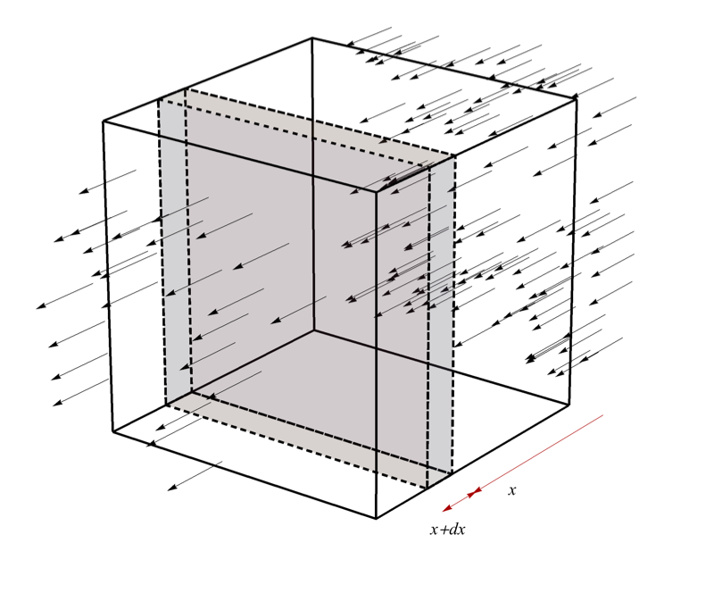Consider a beam of light traversing a material, as shown in the figure. Let the sample have a thickness $L$ and an atomic density of $n$. The photon-atom interactions cause photons to get absorbed by the material. So if the number of photons at a depth $x$ is $N$, then a quantity $dN$ will be absorbed in the next infinitesimal thickness $dx$. Using equation Equation 19 we can write:

\[ \f{dN}{N} =-\sigma n dx \tag{21}\]

Where $\sigma$ is the photon absorption cross-section of an atom. The negative sign is necessary because $N$ is decreasing.

It follows:

\[\begin{align} \int_{N_{0}}^{N}\dfrac{dN}{N} &= -\sigma n \int_{0}^{x} dx \\ \ie \ln N\;\Bigr|_{N_{0}}^{N} & = -\sigma n\, x\;\Bigr|_{0}^{x}\\ \ie \ln\lr{\dfrac{N}{N_{0}}} & = -\sigma n x \end{align}\]

Rearraning give the famous Beer-Lambert Law:

\[ N = N_{0} e^{-\sigma n x} \tag{22}\]

It is often useful to recast the Beer-Lambert law in terms of intensity ($I$) and the linear attenuation coefficient ($\mu = n\sigma$).

\[ I = I_{0} e^{-\mu x} \tag{23}\]

References

PhET Interactive Simulations. 2025. “PhET Interactive Simulations.” https://phet.colorado.edu/.

Footnotes

A vector can be split into more than two components, but this is usually unnecessary.↩︎
About the weight of a typical apple.↩︎
Acceleration tells us how velocity changes (the speed and/or direction).↩︎
Like charge or spin.↩︎
You do not need a force to keep something moving; it only appears that way because friction usually acts against motion.↩︎
Look up Nother’s Theorem if you like to know more↩︎
Energy cannot be created nor destroyed but can be converted from one form to another.↩︎
Weight is the gravitational force on a mass due to the Earth; $mg$ with $g\approx 9.8\,\mathrm{m\,s^{-2}}$.↩︎
By ‘classical’ I mean that particles are distinguishable. This is a subtle point: two ‘identical’ classical particles can, in principle, be distinguished. With quantum particles, however, this is not allowed: there is no way to tell two electrons apart.↩︎

Force	Angle (\(^\circ\))	Work
Push (\(F\))	\(0\)	\(Fx\cos 0 = Fx\)
Contact force (\(R\))	\(90\)	\(R x \cos 90 = 0\)
Weight (\(mg\))	\(90\)	\(mg\, x \cos 90 = 0\)
Friction (\(f\))	\(180\)	\(f x \cos 180 = -fx\)
Total work		\((F-f)x\)